Hazards

The “hazard” is what causes harm to items of interest: in this case, a coastal storm event. The coastal storm event hazard is typically described in terms of frequency, water level, wave parameters, uncertainty, and extent. 

The present configuration of the SCT allows for display of probabilistic still water level hazard information from the Coastal Hazard System (CHS) for the following regions: Louisiana (LACS), Texas (CTX), North Atlantic (NACCS), and the South Atlantic including Puerto Rico and the US Virgin Islands (SACS; USACE 2024).  The figure below shows the areas with available datasets in CHS.  The probabilistic still water level hazards are represented by graded colors corresponding to depths above the topographic surface for a given Annual Exceedance Frequency (AEF) as described in 'Derived Datasets' section.

USACE (2024) provides high fidelity tropical and extratropical coastal storm-related hazards, such as still water levels, winds, and wave characteristics, and corresponding storm event frequencies and hazard uncertainties. Example output hazard curves from the CHS SACS regional study are provided below for still water level and significant wave height for Virtual Gauge 32484.  Details about the underlying modeling and statistical methods used to develop the CHS are also provided by USACE (2024), and the synthetic tropical storm tracks underlying the CHS are visualized in below figure.   It is expected that hazard information for the Great Lakes will be available starting in 2024, with all Great Lakes study areas available in 2025.  These data will be added to the SCT as available.   There have been no commitments by USACE to perform a regional modeling study to support the development of the CHS for the for the Pacific Basin.  Should this effort proceed then the CHART SCT will incorporate the data as they become available and/or seek alternative data sets.

For each regional study, excepting LACS and CTX, simulations included a representation of ‘base’ sea level conditions representative of present-day ocean levels or those based on the present tidal epoch (1983-2001; NOAA, 2024) plus additional simulations to represent future sea level change (SLC) conditions.  Each study, again excepting LACS and CTX, include both tropical and extratropical storm events to characterize wave and water level hazards.

Study regions with low amplitude tide ranges (CTX, LACS) did not include representation of tides in synthetic event simulations but did perform post-processing techniques to include tide in output statistics. Those regions with higher tide ranges (SACS, NACCS) represented tides by various methods (see individual study reports found at USACE, 2024).  The LACS study included several representations of river discharge values for both the Mississippi and Atchafalaya Rivers to account for the variation in hazards resulting from varying storm surge and discharge combinations.  No other regional study considered variations in riverine discharge values.

Statistical analyses performed for each regional study followed the Joint Probability Method (USACE, 2024), producing hazard values and their uncertainty for discrete AEF values.   

Topographic Data 

The ADvanced CIRCulation (ADCIRC) model grids used for regional CHS studies were the source of topographic information supporting frequency-input which requires differencing the first-floor elevation of an asset with the still water level hazard elevation.  Similarly, hazard depths are derived by differencing the grid elevation with the still water level hazard elevation.  The SCT serves this information to the user from a static, precomputed dataset thus no topographic information is required from the user.

Hazard Data

Behind the hazard data is the Adcirc mesh. A mesh is defined by nodes and triangles. See image below for illustration. Each black dot in the image below represents a node. A node is defined as a point in Lattitude and Longitude and also has an attribute of a node id as well as a ground elevation. Triangles are defined in the database as elements. Each element is composed of 3 nodes that make up a single triangle. 

The output from CHS for LACS, CTX, NACS, and SACS were provided in HDF format. Each region requires at least two HDF file formats, one is the spatial data of the mesh itself, the other is the hazard data associated with that mesh. Each region has a specific mesh it is designed to work with. The tables in the mesh file are the Nodes table and the Elements table.

The Nodes table contains the node id, location and elevation of each node in the mesh.

The Elements table contains the element id, and the three nodes that make up the element. 

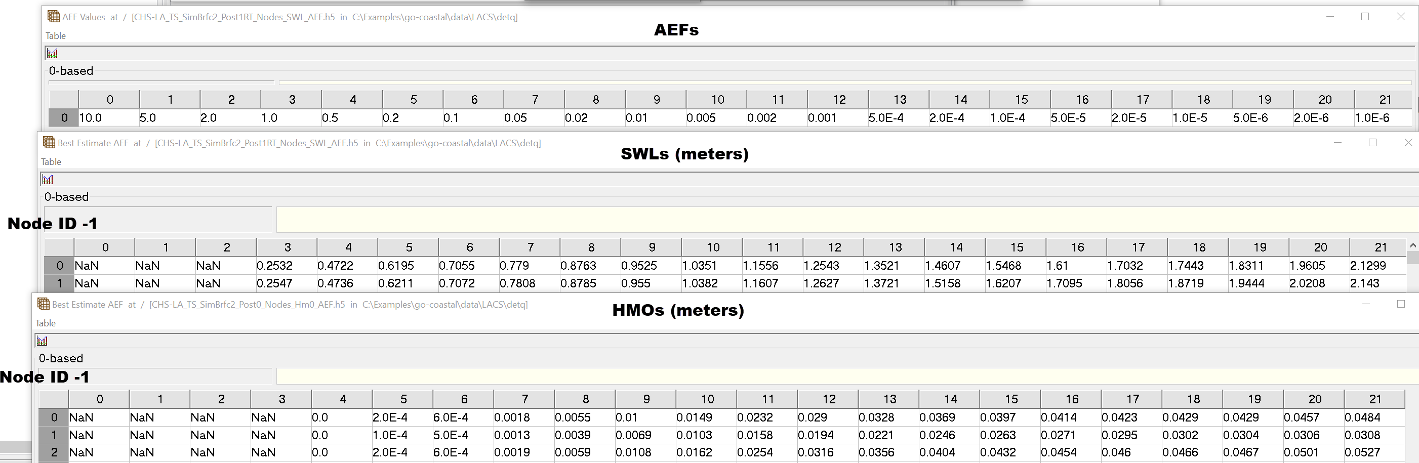
In a separate file specific to a region and a sea level scenario is a set of tables describing the Annual Exceedence Frequency for each column in the database, as well as a table of Still Water Levels (SWL) and Hm0 values. The SWL values and Hm0 values are organized to follow the frequencies by column, and the node id by row (node id's are 1 based index, so the node id - 1 correlates to the row number in the datasets):

Through these tables each node can be associated with the hazard information.  Each node is then associated with each Element to create a set of triangles each referencing the hazard data at the node level. 

Querying Hazard data for a point location

While reading in each element in the mesh with the associated hazard information a bounding box rectangle is defined for each Element, see the blue boxes in the image below. The element is added as a reference to an entry in an R Tree. The R tree is a structure for searching for geospatial data based on bounding boxes. Each query level in an R Tree is a combination of bounding boxes for the query level below. This allows for a quick spatial search to the elements that might contain a point. The benefit of this data structure is to quickly identify the appropriate element that a query point (see green dot in image below) resides within. The final query level for the R tree contains up to 8 Elements that might contain the prospective point. Those 8 elements are each independently queried to determine if the point is contained. 

Only one element will contain the point. For the element that contains the point, the nodes define the frequency based hazard for each node. From there Barycentric interpolation allows the SWL, and Hm0 to be transferred to the point based on the spatial proximity of each node relative to the query point.

The nodal information is then used to assign depth and wave height to each query location.

Damaging depth is defined as SWL + min(.55*SWL, .703*1.6*Hm0)

Derived Datasets

The logic defined above is then utilized for computing the damaging depth at any asset in the consequences calculation or for generating visualization aides such as depth grids.

To compute depth grids query points are generated every 10 m, and are added to a cloud optimized geotiff for each frequency. A gridded result is created for each AEF and SLC scenario. 

References

NOAA, 2024. "Tides and Currents."  Website hosted by Center for Operational Oceanographic Products and Services. National Ocean Service. National Oceanic and Atmospheric Administration.

https://tidesandcurrents.noaa.gov/. Accessed 07 May 2024. 

USACE, 2024. "Coastal Hazards System, V2.0." Website hosted by the Engineering Research and Development Center. https://chs.erdc.dren.mil/Home/. Accessed 07 May 2024.