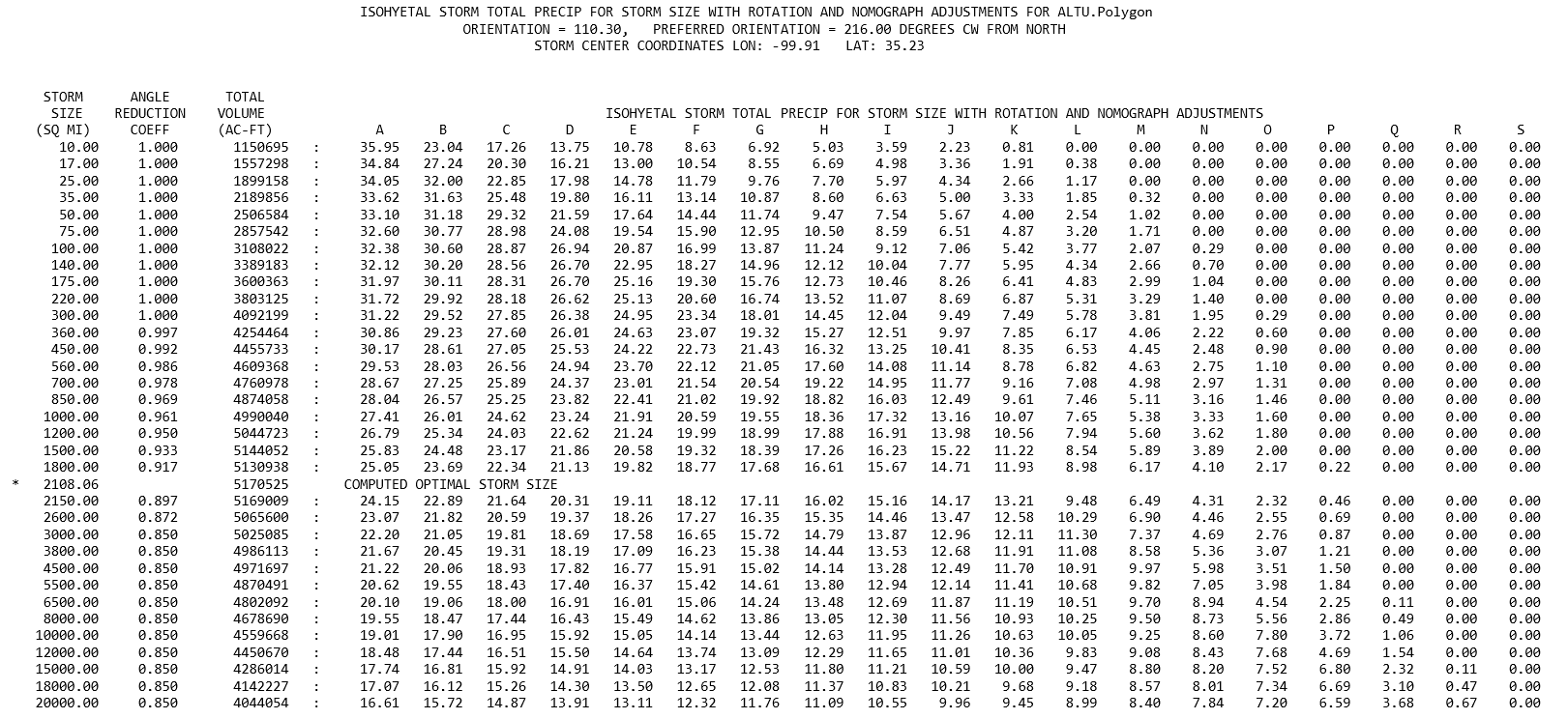
When the storm optimization compute option is selected, the optimized storm size results follow the starting conditions output. The optimization output summarizes the computations that are performed for determining the optimal storm size for the selected location and orientation. The following sample output illustrates the compute results summary for all the storm sizes.
To compute the optimal storm size, a depth-duration curve is created for a specific storm size using the sampled and smoothed Depth-Area-Duration curves, like the curves in the following example figure.

Next, the depth-duration curves for each of the isohyets (A through S) are adjusted using the 6-Hour Nomographs along with the appropriate storm orientation adjustment factor. This storm is then applied to the polygons in the shapefile to compute a total basin precipitation volume. This results in a single trial point on the curve shown in the following figure. Several storm size versus precipitation volume computations are performed to create the curve shown in the following figure.

Using the curve points from the standard storm sizes described above, the optimal storm size is determined by constructing a curve using a Catmull-Rom spline curve fitting algorithm.
In the example in the figure above, the maximum storm size of around 2109 square miles is found through a bisection search algorithm. Normally, the plugin will only compute enough size alternatives to define an adequate curve for determining the optimal storm size, which requires at least three trials on each side of the computed maximum similar to what is shown in the above spline curve figure.
Referring to the summary table at the top of the page, the row with the asterisk in the leftmost column denotes the optimal storm size. Quite often, the optimal storm size is one of the computed storm sizes. But, since the optimal storm size in this example falls between the standard storm sizes from the nomograph tables, a final computation is performed by interpolating between the standard storm sizes to adjust the isohyets proportionally.
The angle reduction coefficient shown in the table is computed from the storm orientation adjustment factor nomograph as shown in the next figure.
