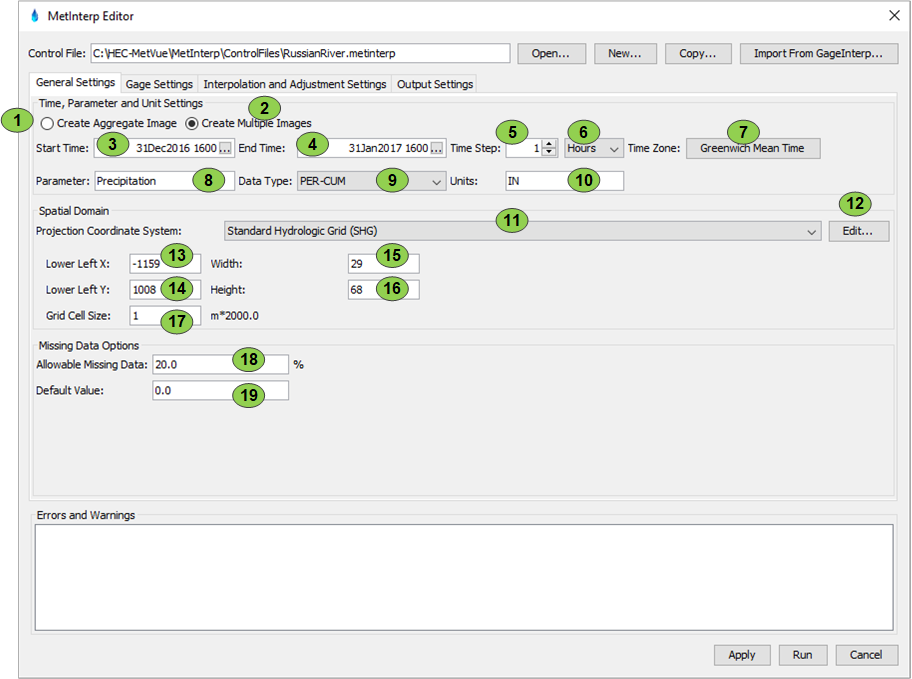
| 1 | Create aggregate image radio button sets MetInterp to create a single aggregate image from the data. |
| 2 | Create multiple images radio button sets MetInterp to create an image for each time step specified in the settings. |
| 3 | Start time field allows for specification of the start time in the computations. When creating aggregate image, this is the start time of the image. When creating multiple images, this is the start time of the first image. |
| 4 | End time field allows for specification of the end time in the computations. When creating aggregate image, this is the end time of the image. When creating multiple images, this is the end time of the last image. |
| 5 | Time step amount. In combination with the time step unit, defines the time interval between images when using the Create Multiple Images option. |
| 6 | Time step unit. In combination with the time step amount, defines the time interval between images when using the Create Multiple Images option. |
| 7 | Time zone button launches a time zone selector for specifying the time zone of the output data. |
| 8 | Parameter is a description of the type of data. This specification is unrestricted, but should represent the data. Common parameters are Precipitation and Temperature. |
| 9 | Data type selection describes how the output data should be distributed over the time interval between images. For example, PER-CUM is period cumulative data typically used for precipitation. INST-VAL is instantaneous values used when instantaneous temperature measurements are used. Note that careful attention should be paid to the input time series, as not all data type conversions are possible. For example, if the input time series is INST-VAL, conversion to an output data type of PER_CUM is not possible, and in this configuration an error will be issued. |
| 10 | The units in which the output data should be written. This is unrestricted, but should be a reasonable description of the output data units. |
| 11 | The output coordinate system |
| 12 | Button to launch a coordinate system editor. This allows for custom definition of a coordinate system. |
| 13 | Output grid lower left cell x index. This index is based on the coordinate system, considering the cell size. For example, this field is populated in the image above with -1,159, which is -231,8000 meters (-1,159*2,000 meters) from the x origin of the specified coordinate system. |
| 14 | Output grid lower left cell y index. This index is based on the coordinate system, considering the cell size. For example, this field is populated in the image above with 1,008, which is 201,600 meters (1,008*2,000 meters) from the y origin of the the specified coordinate system. |
| 15 | Output grid width in number of cells. In the image above, this is the 29 grid cells, so the width of the grid is 58,000 meters (29*2,000 meters). |
| 16 | Output grid height in number of cells. In the image above, this is the 68 grid cells, so the height of the grid is 136,000 meters (68*2,000 meters). |
| 17 | Resolution of the grid cells in the coordinate system units |
| 18 | Percent of allowable missing data in the time window, beyond which the gage will be removed from the analysis. |
| 19 | Default value for replacing missing values. |