Download PDF
Download page Data Screening and Estimating.
Data Screening and Estimating
Many data sets contain erroneous values, which must be corrected before performing mathematical operations with the data. HEC-DSSVue provides some limited screening criteria, allowing values to be declared as 'missing', and/or quality flags to be set. This workshop demonstrates three of the four mechanisms available to identify and replace invalid data:
- Screen Using Minimum and Maximum
- Screen with Forward Moving Average (not used in this workshop)
- Manual editing of values inside Tabulation window
- Estimate Missing Values
Task 1. Select and View Data
- Start HEC-DSSVue and open “TimeSeriesMath.dss”
- Click the Set Time Window button and select No Time Window if it is not already selected. Close the Set Time Window dialog.
- Select View → Condensed Catalog from the menu bar. In the absence of a time window, this makes subsequent operations on a pathname apply to all the records, regardless of the D-part.
- Select View → Unit System → As Stored from the menu bar, to avoid inadvertent unit conversions when writing Math Functions results back to the database.
- Select the data set named
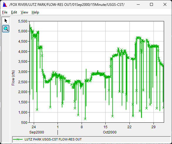
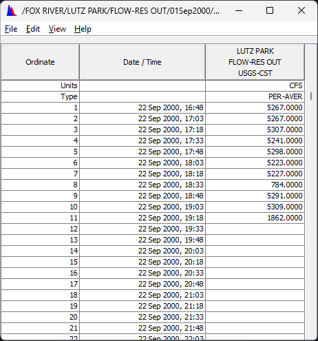
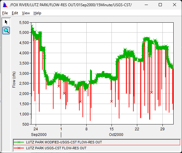
/FOX RIVER/LUTZ PARK/FLOW-RES OUT/22Sep2000 - 31Oct2000/15Minute/USGS-CST/ - Plot and tabulate the data.
- Notice the plot indicates the shape of the good data but has lots of bad data points.
- Notice the table shows that the data is offset three minutes into every 15-minute interval..
These data were produced by a very old USGS Acoustic Velocity Meter. Each minute it made an instantaneous measurement of mean velocity across the channel, which it multiplied by cross-sectional area to calculate flow. Every 15 minutes it applied some very coarse quality-control procedures, averaged the samples, and reported the resulting flow to the USGS.
Task 2. Screen Data
In situations where the actual data changes gradually, individual fluky values can be easily screened out using a “moving average” technique. However, this gage is located a short distance downstream of the Lake Winnebago outlet structures and hydropower facilities. Abrupt flow changes typically indicate gage malfunction but can be difficult to distinguish from actual variations due to gate movements or generating adjustments.
- Launch the Math Functions dialog from the tool bar or menu bar.
- Choose the General tab and Screen with Forward Moving Average operator.
- Your engineering judgment and experience with this gage suggest that the flows cannot realistically change more than 500 cfs in an hour (four 15-minute periods).
- Screen the data set using the parameters shown in the figure below. (Be sure to click the Compute button)
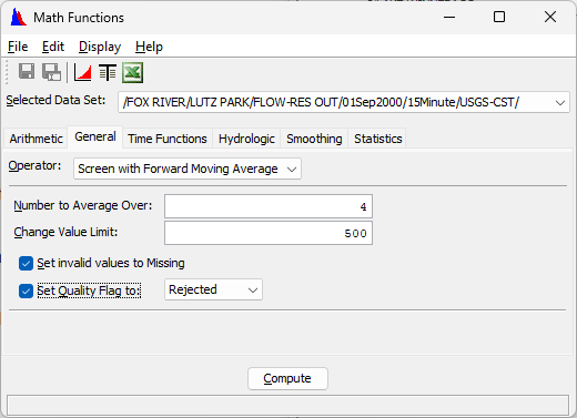
- Screen the data set using the parameters shown in the figure below. (Be sure to click the Compute button)
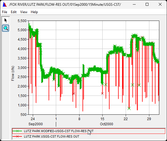
- Plot and tabulate your computed data to review the changes.
- Try selecting 'Original Data with Computed' under the Display menu and re-plotting the data.
- Question 1. If the original curve covers up the “modified” curve in the plot, how can you switch order so that the revised curve is plotted on top of the original?
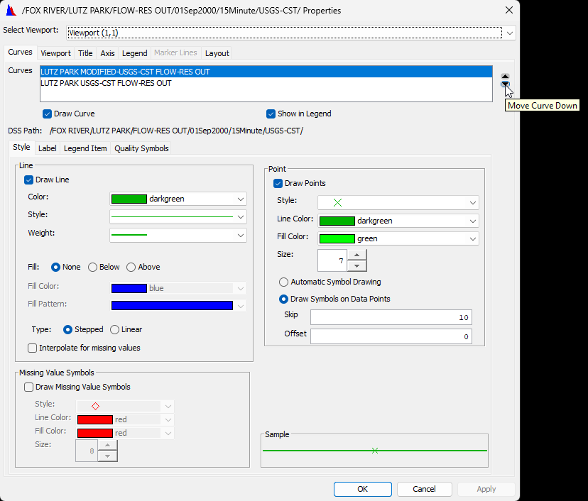
- Go to the "Edit" button on the ribbon and select "Plot Properties..."
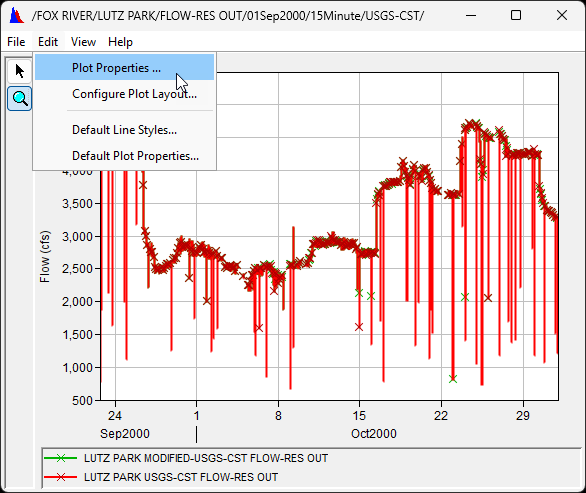
- Use the arrows to the right to change the order of the curves
- Alternatively, you can click on the desired data set in the legend to highlight it.
- Go to the "Edit" button on the ribbon and select "Plot Properties..."
- Select View → Quality → as symbol and View → Quality → as hex from the table menu bar.
- Note the three different quality flags associated with the “modified” data?
- 0000 0003 (hex) or empty cell (symbol) means okay value,
- 0000 0005 (hex) or M (symbol) means missing before the test.
- 0000 0011 (hex) or R (symbol) means rejected by the test.
- Note the three different quality flags associated with the “modified” data?
- Look again at the plot and note that many dubious values persist.
- The revised data is still unfit for use in computations.
- Perhaps a more aggressive screening test is needed.
- Leave the existing plot open for subsequent comparisons
- Re-screen the data using a change value of 200 cfs over four 15-minute periods.
- Select Edit → Restore Original Data from Math Functions menu bar and verify that when you plot the data that only the original pathname appears.
- Modify the Change Value Limit value to 200 and click the Compute button.
- Review the results by plotting and tabulating.
- Question 2. Did the stricter test reject any additional data (bad or good)?
- Yes. You can tell by comparing the 500 cfs screening (left) with the 200 cfs screening (right) that the bad point around the Oct 9 is no longer included in the screened data, but some good values in the steep transitions were also rejected.

- Since we had difficulty effectively screening the data using Screen with Forward Moving Average, let's try a different method.
- Restore the original data again (Edit → Restore Original Data) and verify that when you plot the data that only the original pathname appears.
- Screen the data using the Screen using Minimum and Maximum operator with the values shown in the figure below.
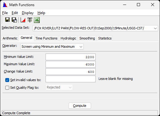
- Plot and tabulate your computed data to review the changes.
- Question 3. Does the revised data look ready to for use in a computation? Why or why not?
Not ready yet because calculations (and models) generally require all values to be present. The missing values will need to be addressed in some way.
Also note the upward-spike on 9Oct2000, and a block of dubious data on 25Oct2000 still remain after the initial screening,.
- Save the results so far using File → Save As from the Math Functions dialog menu bar or the Save As icon on the Math Functions dialog tool bar.
- Save with the F part name of USGS-CST-REV
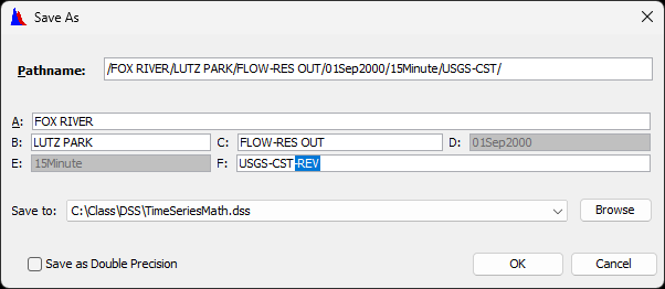
- Close the Math Functions dialog.
- Save with the F part name of USGS-CST-REV
- Manually clear bad values on October 9.
- From the HEC-DSSVue window, clear any previously selected pathnames, and tabulate your revised data.
- From the table menu bar:
- Select Edit → Allow Editing
- Make sure View → Date with 4 Digit Years is selected
- Make sure View → Date and Time Separately is not selected
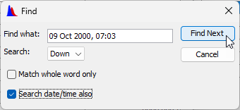
- Scroll down to the values for 09 Oct 2000, 07:03 (you can also use Edit → Find... or F3 to search for the date/time)
- Highlight the rows of 09 Oct 2000, 07:03 and 09 Oct 2000, 07:18.
- Right-click on the selected values and select Clear.
- Save your changes to the same pathname (File → Save or Ctrl-S) and close the table.
- Use focused time window to screen out bad values on Oct 25.
- Click the Select Time Window button on the HEC-DSSVue window and set the time window as shown:
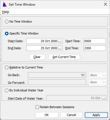
- Plot and tabulate the data to show that flows below 4500 cfs in this time window are likely bad
- Launch the Math Functions dialog using the recently created/revised data set.
- Since the time window is set, the operations are confined to data for 25Oct2000.
- Execute the Screen Using Minimum and Maximum with the Minimum Value Limit of 4500.
- You can leave the other value fields blank so that no maximum value or change limit is imposed.
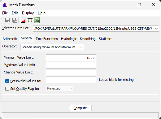
- You can leave the other value fields blank so that no maximum value or change limit is imposed.
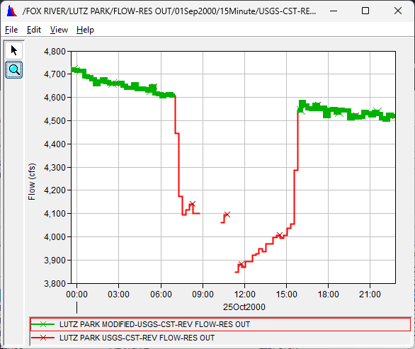
- Plot the modified and original data to verify the results of the operation.
- Save the data back to the same name and close the Math Functions dialog.
- Click the Select Time Window button on the HEC-DSSVue window and set the time window as shown:
- Verify the results so far.
- Clear the time window in HEC-DSSVue, and plot the data.
- All suspicious values should be gone.
- Close your plot.
Task 3. Fill Gaps in Data
- Lauch the Math Functions dialog with the revised Lutz Park flows.
- Select the Estimate Missing Values operator on the General tab.
- Execute the computation with value of 96 to prevent estimating more than a day's worth of 15-minute values

- Plot and tabulate the new data set, verifying that all of the missing values have been filled in.
- Save your data.
- Close the math window if it is still open.
- Your data technician passes by and points out that cleaned up data already exists in /FOX RIVER/LUTZ PARK/FLOW-RES OUT//15Minute/USGS-CST-FIXED/.
- He thinks it’s great that you walked a mile in his shoes, but really, you should just use the “fixed” version provided by an experienced professional, pointing out that:
- The values on Oct 25 were valid and should not have been screened out
- That the parameter type must be "INST-VAL" according to an arbitrary but long-standing convention.
- He thinks it’s great that you walked a mile in his shoes, but really, you should just use the “fixed” version provided by an experienced professional, pointing out that:
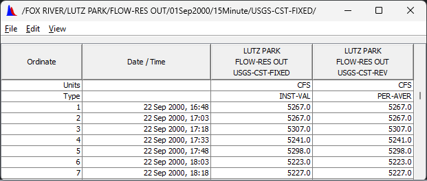
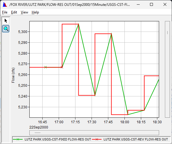
- Plot and tabulate your "-REV" data vs the "-FIXED" data.
- Question 4. Does re-defining the parameter type to "INST-VAL" actually change anything?
Yes, the meaning of the timestamps has changed. What was previously the end of an averaging period is now the time of an instantaneous observation.