Download PDF
Download page HEC-DSSVue Utilities & Tools.
HEC-DSSVue Utilities & Tools
Files for this workshop:

Introduction
The intent of this workshop is to demonstrate the various utility functions in HEC-DSSVue, their purpose and how to use them.
Task 1. Creating and working with Groups
- Start HEC-DSSVue
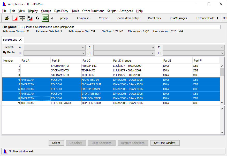
- Open sample.dss
- Find all the pathnames for FOLSOM and select them.
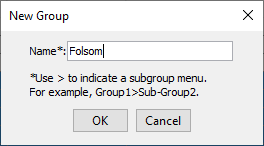
- Create a Group, from the Groups menu
- Name that group “Folsom”.
Question 1: Describe the different functions you can perform from the Group Menu.
Get – Put the data sets in the selection area
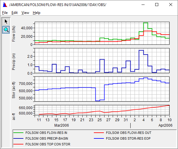
Plot – Plot the data sets together, in one plot
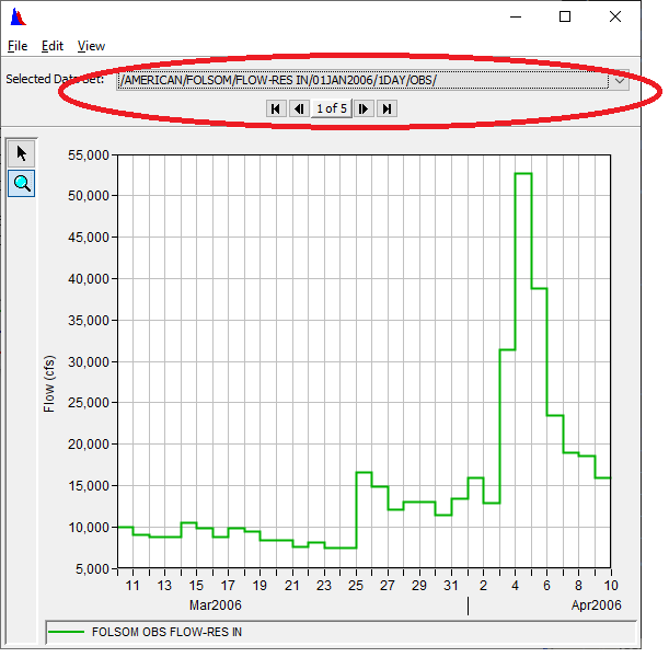
Plot Individual – plot each data set one at a time
Tabulate – tabulate the data sets (in one table)
Math – perform math functions on the data sets
Question 2: What is the difference between Group -> Plot and Group -> Plot Individual? Run them both.
Plot plots all the data sets in one single plot.
Plot Individual plots each data set in a single plot and allows you to scroll through the plots.
Question 3: Is a time window associated with a group?
Yes, if a time window is set when the group is created. You can change or delete the groups time window from the Manage dialog.
If you don't have a time window set the group will not have a time window.
6. Go to Manage.
Question 4: What can you do in this dialog? What are the items under the Edit menu?
This dialog allows you to manage all the groups you have created. This includes deleting or adding pathnames; changing file locations, time windows, or the group name; and deleting groups.
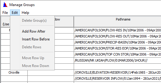
The items under the edit menu include deleting and adding rows (for pathnames), and rearranging the order of the pathnames. You can also delete a group from the edit menu.
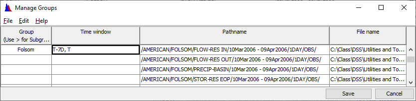
Question 5: Say you wanted to analyze the last week of data for the datasets in the Folsom group. However, you don’t want to have to change the time window every time you access the group. Set this up and describe how you did it. Note: There is more than one way to do this. What happens if you try to plot the group?
You can set a relative time window on the first line of the group to “T-7D, T”, which is means the start time is the current time minus 7 days and the end time is the current time.
Nothing will plot because no data is within the set time window.
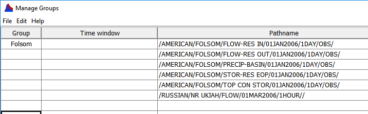
7. From the Manage dialog, add the flow at Russian River gage near Ukiah to the Folsom Group you created.
- The pathname is /RUSSIAN/NR UKIAH/FLOW/01MAR2006/1HOUR//.
8. Click Save and close the dialog box.
- To ensure the records were added use Get from the Groups menu to show the records in the selection window.
Task 2. Water Year
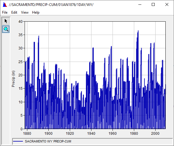
Period of record daily incremental precipitation for Sacramento is in sample.dss.
- Find it and plot it.
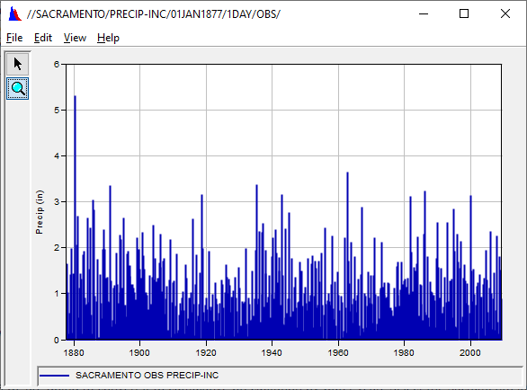
Question 6: Can you make any sense of it?
Not too much sense, because it covers some 130 years of daily data. You can see that it is rare if it rains more than 3 inches in one day. Only once has it rained more than 4 inches in a day.
The data is incremental, and it’s hard to analyze in this form. To make the data easier on the eyes we are going to convert it to cumulative precipitation by water year.
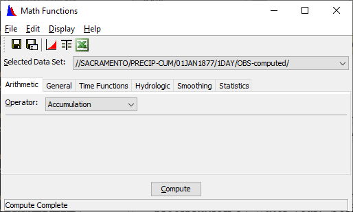
2. Select the Sacramento incremental precipitation record and open the Math Functions dialog.
3. Go to the Arithmetic tab and select the Accumulation Operator.
4. Press Compute.
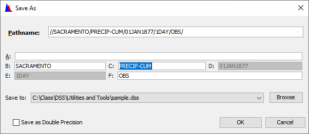
5. “Save as” the computed data set with a C Part of PRECIP-CUM.
6. Close the Math dialog and then plot the data from the main screen.
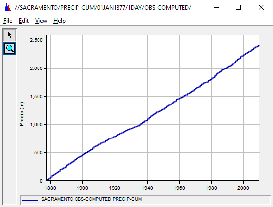
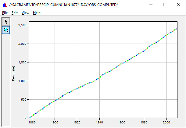
Question 7: What is the plot showing now? Is it any more helpful than before?
It increases monotonically from 1877 to 2009 to a value of about 2,400 inches. Still not too useful for analyzing the data.
We’d like the precipitation to start at zero at the beginning of the water year (October 1 in California).
7. Select the data set that you just saved.
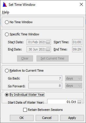
8. Open the Time Window dialog and select By Individual Water Year.
- Be sure the start of the water year is 01 Oct.
9. Press OK.
10. Go to the main screen and select plot.
- If the legend is dominating your screen right-click on the legend and select 'Hide Legend'.
Question 8: What has changed with the plot?
The plot is still cumulative throughout the period of record, but now it has colors with each year is displayed as a separate data set.
11. Close the plot.
12. Go to the Display menu and then Display Data Options and select Normalize.
- Check the message bar at the bottom of the screen to verify you have water year and normalize selected.
13. Plot the data again to see what has changed.
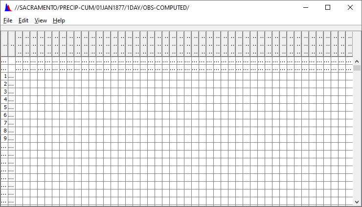
14. Now tabulate the data.
- Your table should be so cramped that you cannot see any data in it… that’s ok.
15. In the table menu, go to File and select Save As….
- Set the F part to WY.
16. Save your data.
17. Plot your data.
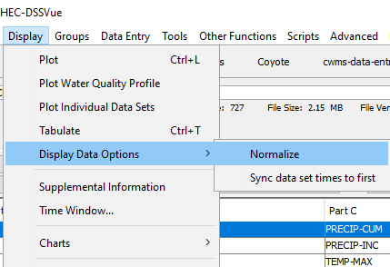
Question 9: What do you see now?
The table was completely un-readable; however, all the data was saved with the first value for the water year starting at zero. I had to turn off the legend on the plot to see anything… and after that, it looked like magic rocks. I turned off the water year for the time window and got the plot below.
Compare the precipitation for a few years.
18. Set the View to Pathname Parts
19. Filter F part to be WY.
- You should now have a list of individual records for each year.
- Be sure that you have Water Year still set.
20. Go to the Display Data Options and select Sync data set times to first.
- It doesn’t matter if Normalize is on or not, as we have already normalized it.
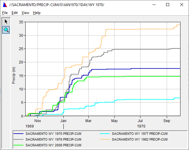
21. Select pathnames for the following years:
1970; 1977; 1978; 1982; 2008
22. Plot the data.
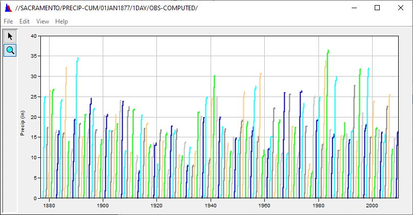
Question 10: Describe what you see. What year was the wettest and which was the driest? What were the totals for those years? What season does it rain? What season does it NOT rain?
This shows hyetographs for the different water years – an easy way to compare the years. 1982 was the wettest, with a total of 34 inches. 1977 was the driest with only 7 inches. It rains in the winter time, November through March. It doesn’t rain in the summer (July – September).
Task 3. Duplicate and Compare
- Reset the display options and change the time window to No Time Window.
- In sample.dss, select all of the OAKVILLE records
- Bring up the Duplicate dialog
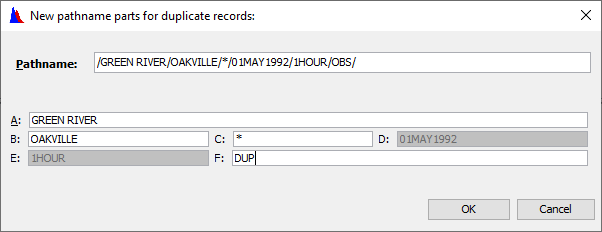
You can bring this dialog up from the Edit menu, or right clicking on the select pathnames and selecting Duplicate.
Question 11: Why can’t you change the D or E parts? How could you (legitimately) if you really wanted to?
These parts are the time dependent parts that the data relies on. You cannot change the date simply by giving it a new date part, nor change the time interval by providing a new E part. If you somehow forced this, the data would be all messed up.
You can change these by using the Time Functions tab in the Math Functions module, and selecting “Shift in Time”, and “Change Time Interval”.
Question 12: What does the “*” mean for the C part? What would happen if you changed that? (Don’t do it!)
The “*” indicates that there are different part names for the records selected (e.g., ELEVATION, PRECIP-INC) If you changed that part, then the data sets would have the same name and they would write over each other… not a good thing.
4. Change the F part to DUP
5. Press OK
Question 13: Is there any difference between the duplicated and original records? How do you know?
No difference – it’s duplicated data. I can be sure by using the compare function…also by comparing plots or tables to get a quick idea.
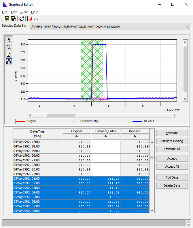
6. Graphically edit the OAKVILLE ELEVATION that you duplicated.
7. Remove the block spike on May 5 by drawing a free hand line using the multi-point Edit tool.
- When it looks good click 'Accept All'
- Save the data.
ref: https://www.hec.usace.army.mil/confluence/dssdocs/dssvueum/display-and-editing/graphical-editing
8. From the catalog select your edited data and the original data set
9. Go to the Tools menu
10. Select Compare -> Data Sets.
11. Select Show Full Table is the dialog that appears.
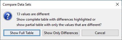
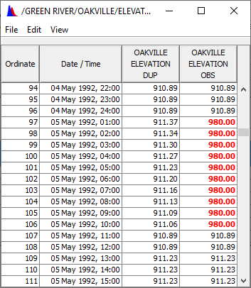
Question 14: What happened?
A table showing the differences highlighted in red, or a table with just the differences is shown.
12. Now try Compare -> Data Sets with Options
13. Set the Percent Difference to 15%.
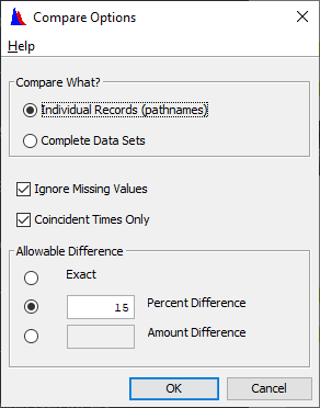
Question 15: What happens when you compare now?
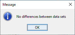
Question 16: What is the smallest percent change that you can use so that DSSVue will find no difference in the datasets?
The percent difference between 980 and 910 is about 7-8 %. When selecting 8% no differences were shown between the data. When selecting 7% differences were shown.
Task 4. Search for Values
- Filter by C-Part of "PRECIP-INC", an E-Part of "1HOUR", and an F-Part of "OBS"
- Select all the pathnames
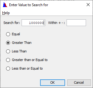
- Use the Search for Value function to answer the following questions:
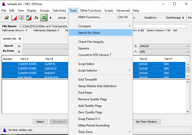
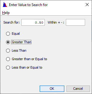
Question 17: Are there any precipitation records in the DSS file that have more than 0.50 inches in an hour? When and where?
You need to use the search by parts option to select only records with C parts of PRECIP-INC, E parts of 1HOUR and F parts of OBS (so we don’t search the duplicates)… otherwise you would be searching the wrong data sets.
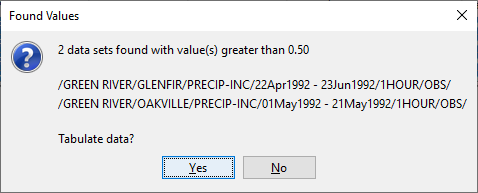
Glenfir on the Green River had a value of .83 on 11May1992, and .64 on 12May; Oakville on the Green River recorded a value of .71 on 03May1992.
Question 18: Are there any flow records that have values over 1,000,000 cfs? (All flows are in cfs in this file.) When and where? Note: There are several different flow types. How can you search for all data sets containing flow in one step? Hint - look in the View menu.
You can use the Search Pathnames option, which will look for FLOW anywhere in the pathname. That way, you’ll get FLOW-RES IN as well as FLOW-RES OUT was well as FLOW.
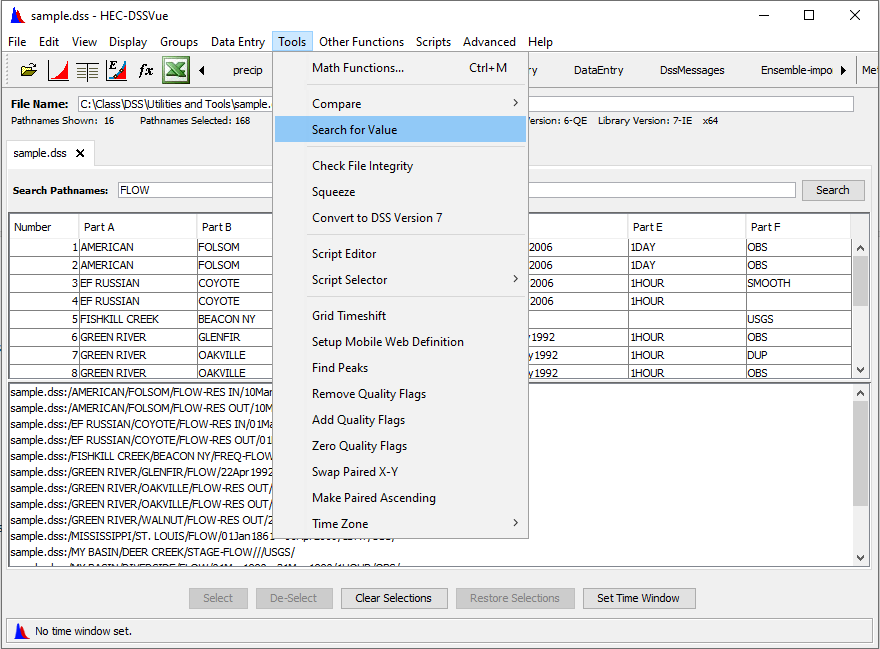
One data set was found – the Mississippi at St. Louis on 10-12 June 1903.
You can quickly find the highlighted differences by either pressing the F3 key, or selecting Next Difference from the Edit menu.
Task 5. Undelete Records
Question 19: Delete your duplicated records. Has the file size changed? Can you tabulate any of the deleted records?
No, the file size remained the same (in my case it was 2.62MB). I can see the size under the file name, or I can use Windows Explorer to check it. After I deleted the records, the catalog refreshed and they didn’t appear – so there is nothing there to try and tabulate.
- Open the Undelete dialog by going to the main Edit menu
- Selecting Undelete -> Select…
Question 20: What did this display? How many records are available to undelete?
This displayed a dialog with checkboxes and pathnames that are the ones that I deleted earlier. There are 6 of them.
3. Undelete the OAKVILLE ELEVATION that you edited.
Question 21: Can you tabulate it now? Did the file size change?
Yes, that pathname reappeared in the catalog and I could tabulate it. No, the file size didn’t change.
Task 6. Check File Integrity and Squeeze
- Run the file check command on sample.dss by selecting Tools -> Check File Integrity.
Note: HEC-DSS is designed in a way that it is difficult for a file to be damaged by software or users. However, files on PC can be damaged. File Check is a through test to check for any damage. It will not check for bad values, just broken addresses and the like.
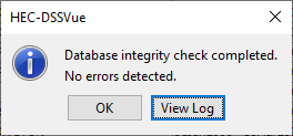
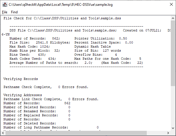
Question 22: Are there any errors in the file? View the log file. What does this tell you?
This log file gave me information about internal statistics, and numbers of records, as well as 0 Errors found.
2. To demonstrate the file size reduction capabilities of the squeeze function let’s take a look at the file sizes before and after a squeeze.
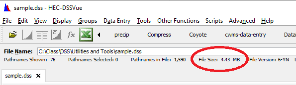
Question 23: First, what is the current file size of sample.dss?
3. Now select all the records in the file
- Duplicate them with an F Part of DELETE
- Duplicate them with an F Part of DELETE
Question 24: What is the file size now?
4. Delete all the records that you just created
- This is simulating a user editing data, performing functions and creating new datasets which creates inactive file space
Question 25: What is the file size now?
deleting records did not change the file size.
5. Squeeze the file. Tools→Squeeze
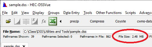
Question 26: What is the new file size?
My file size dropped to 2.48 MB, according to the size on the main window
Question 27: Try opening the Undelete dialog. What happens? Why?
There were no records to undelete. This is because the squeeze removed deleted records and other dead space. Squeeze is a little like emptying the recycle bin.
Question 28: Open the file “funny.dss”. funny.dss was being written to when the computer went blue screen (BSOD). Run file check on this file. Are there any errors? How many and what are they? What is the file size?
If the check file integrity on this file crashes HEC-DSSVue application, try squeezing the file and moving on with the workshop.
Something funny is going on with funny.dss. It told me that there were 5 errors and I should squeeze the file to repair it. If you look closely, you’ll see that there are only 2 errors – 2 lost records, but the check found them through different error checking procedures and reported the same error twice. File size is 211KB.
Question 29: Squeeze the file “funny.dss”. Recheck the file integrity. Are there any errors now? What is the file size? Speculate on why it changed so much.
No errors now. File size reduced to 67KB from 211KB! If you look in the log (above), you’ll see156 records had been deleted. This space was removed when the file was squeezed.
The two records that were shown as errors were recovered and can be accessed as normal now.
Task 7. Disk Catalogs and Supplemental Information
- Close “funny.dss”
- Open “sample.dss”
- View the Sorted Full disk catalog from the Advanced menu
Question 30: What information does it give you?
This provides a list of all the pathnames of the records in the .dss file sorted in alphabetical order.
Question 31: Now, say you need a sorted list of pathnames for every record in the catalog with the word FLOW in the C Part. How would you do this?
Might need to enable "Catalog using wild characters" to use this function found in View.
In the Advanced menu, in Catalog to File select Sorted using wild characters. In the dialog box that opens, input “*FLOW*” to the C Part (between the third and the fourth slashes). The “*” on the front and back allow any characters to precede or follow “FLOW”.
Question 32: How many records are in this list? (HINT: you can use excel to help you count)
There are 167 total records in the list.
BONUS Question: Describe another way to get this list.
Go to the View menu, select Pathname List and select Search using wild characters. When you type “flow” in the search box every record that contains the string “flow” will appear in the catalog. From here you could select all pathnames and copy to clipboard.
Question 33: Open the Supplemental Information for the Mississippi River gage at St. Louis. What Type of data is in this record? How many times has it been written? By what program?
The Data Type is Period Average. It has been written a single time by DSSVue.