Download PDF
Download page Normalizing Data.
Normalizing Data
After data sets have been screened, they may still require conversion to a common time-series scale before being used together in computations. In order to calculate hourly reservoir inflow, the data sets for the lake levels and outflows should be normalized to the same hourly intervals.
Task 1. Convert Data to Hourly Intervals
- Clear any time window that may be set and launch the Math Functions dialog with the data set named /FOX RIVER/LUTZ PARK/FLOW-RES OUT/22Sep2000 - 31Oct2000/15Minute/USGS-CST-FIXED/
- Note that this is not the data set you generated previously.
- Tabulate the data from the Math Functions dialog.
- Note that the outflows occur every 15 minutes, at an offset of 3 minutes.
- Subsequent calculations require hourly flows averaged at the top of the hour.
- Select the Time Functions tab and the Min/Max/Avg/…Over Period operator.
- Set the Function Type to Average over Period.
- Set the New Period Interval to 1HOUR.
- Do not save as irregular interval or set an offset.
- The resulting time series will be the average flow for each hour, computed from the original data
- Click the Compute button; plot and tabulate the computed data with the origina.
- Question 1. What is the Type of the resulting data? How does this affect the values computed for the new time interval?
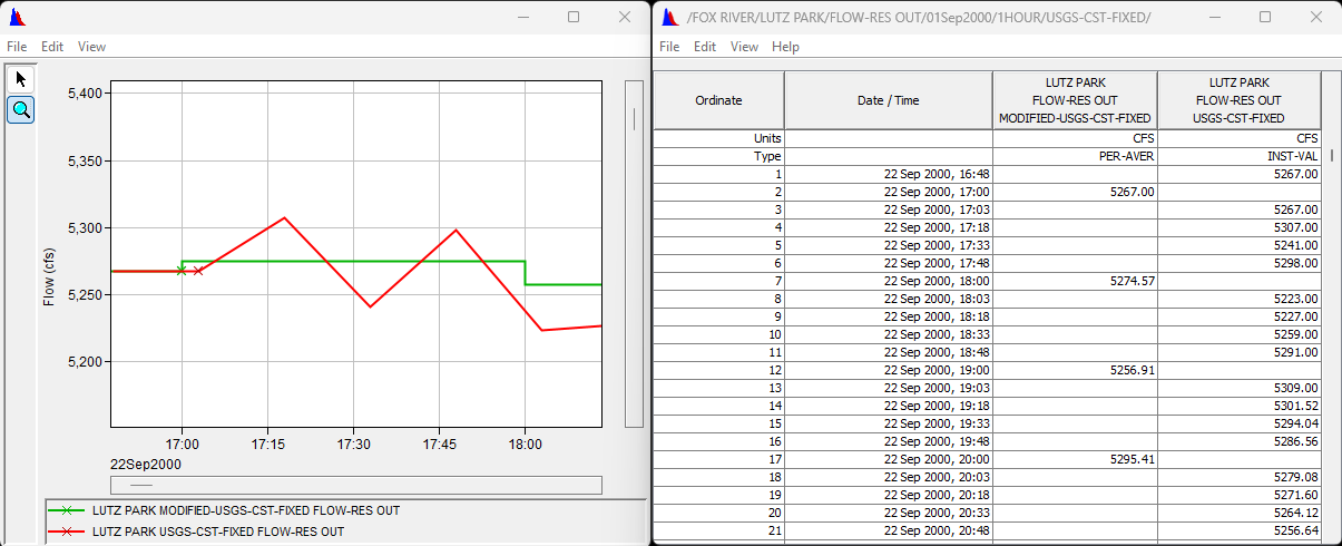
The Type of data generates is PER-AVER. This impacts the computed results due to the fact that we are averaging the data over the period. The averaged data will not be as volatile as the 15-minute data.
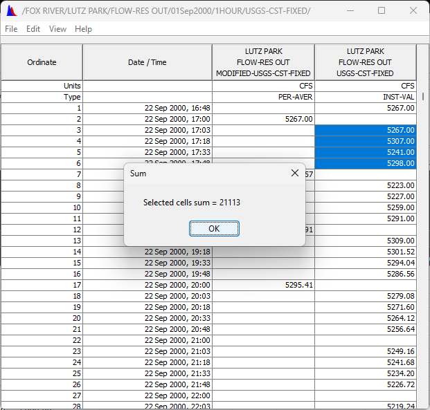
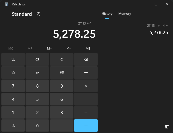
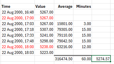
- Question 2. If you average the 4 values immediately prior to the 22 Sep 2000, 18:00 value you get a value of 5278.25 instead of the computed value of 5274.57. Why is there a discrepancy?
Because the 1-hour interval doesn't line up with the 15-minute data, allowing:
- the value at 16:48 to have three minutes of influence
- the value at 17:48 to have only 12 minutes of influence.
In the image below:
- The red values are linearly interpolated from the surrounding values to be at the beginning and end of the interval.
- The Average column contains the mean of the previous and current value multiplied by the number of minutes for each mean.
- The Minutes column contains the minutes for each contribution.
- The result is the sum of the Average column divided by the sum of the Minutes column - or more accurately the sum of the Averages column divided by the interval minutes (\Large{\frac{\sum_{i=1}^{n} \frac{v_i + v_{i-1}}{2} \cdot (t_i - t_{i-1})}{{t_n - t_0}}}}).
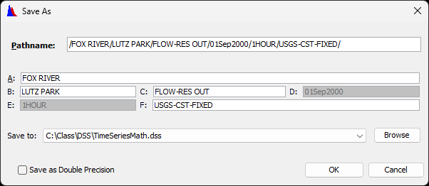
- Save your new data set using the suggested E part of 1HOUR (this will be auto-generated from the New Period Interval value in the Math Functions dialog).
- Close the Math Functions dialog. as well as any plots or tables
Task 2. Interpolation
The two elevation data sets will later be averaged into a mean reservoir level but first must be normalized to hourly data. The irregular Fond Du Lac data set consists of readings taken at the top of each hour, as well as one taken every 4 hours at the satellite ‘shoot’ time.
- Clear any time window that may be set and launch the Math Functions dialog with the data set named /LAKE WINNEBAGO/FOND DU LAC/ELEV/22Sep2000 - 01Nov2000/IR-Month/COE-CST/
- Select the Time Functions tab and the Irregular to Regular operator.
- Select the Interpolate (fill-in values) option.
- Set the time interval to 1HOUR.
- Do not set an offset - the resulting time series will be interpolated at the top of each hour.
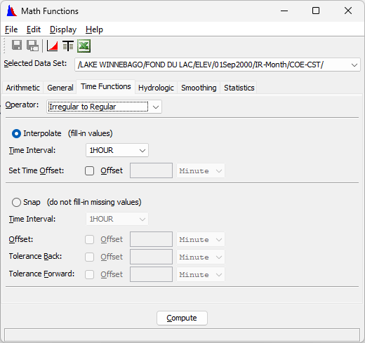
- Click the Compute button.
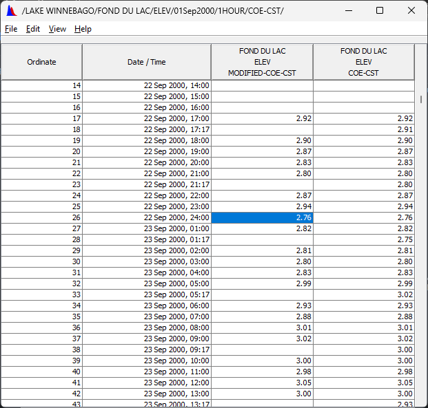
- Tabulate the results to verify that only the top-of-hour values remain.
- Save the modified data using the proposed E part of 1HOUR.
- Close the Math Functions dialog. as well as any plots or tables
Task 3. Snapping
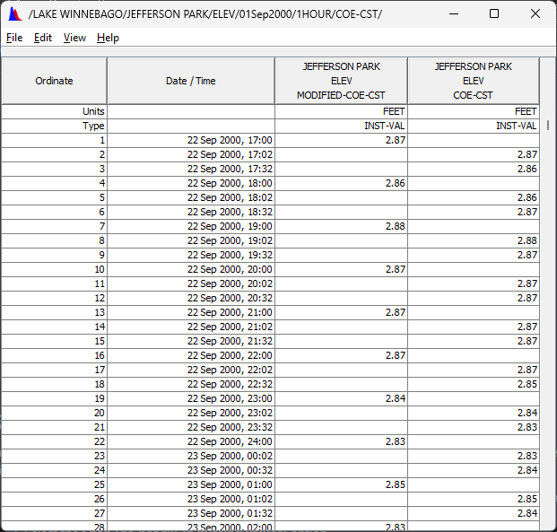
The 30-minute Jefferson Park data set consists of instantaneous readings taken at 2 and 32 minutes past each hour. If simply converted to an hourly interval, the levels at the top of the hour would be linearly interpolated between the values at 32 and 2 minutes. This has the unfortunate effect of attenuating the high and low points. It is preferable to avoid this attenuation by extracting the 2-minute offset readings, and “snapping” them back to the top of the hour.
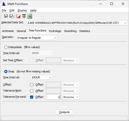
- Clear any time window that may be set and launch the Math Functions dialog with the data set named /LAKE WINNEBAGO/JEFFERSON PARK/ELEV/22Sep2000 - 31Oct2000/30Minute/COE-CST/
- Select the Time Functions tab and the Irregular to Regular operator.
- Select the Snap (do not fill-in missing values) option.
- Set the time interval to 1HOUR.
- Set the Tolerance Forward to 2 Minutes
- Click the Compute button.
- Tabulate the results to verify that only the values originally at a 2-minute offset remain, and that they are now shown with an offset of 0 minutes.
- Save the modified data using the suggested E part of 1HOUR.
- Exit the Math Functions dialog and close any plots or tables.
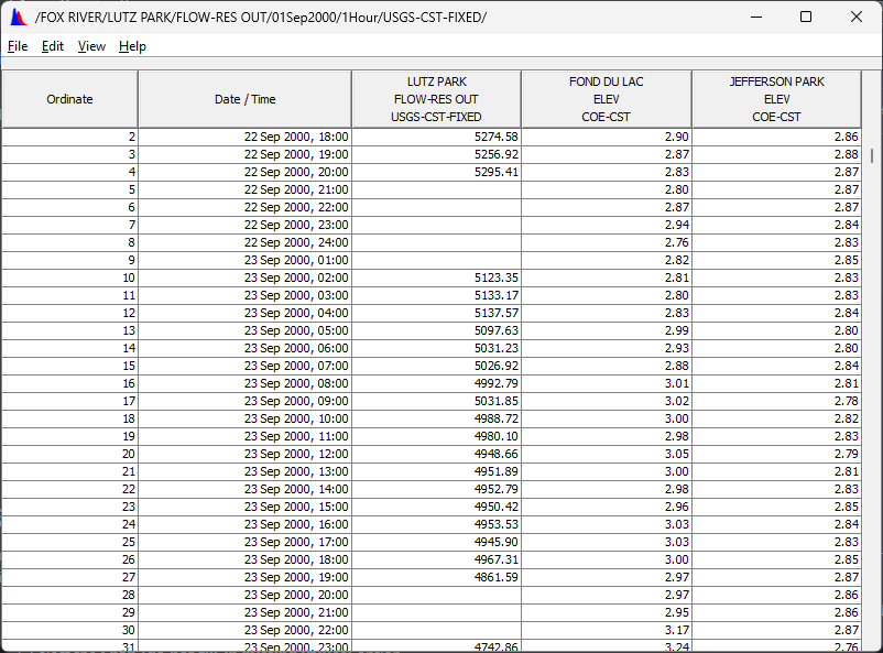
- From the HEC-DSSVue Main Window, tabulate the new hourly pathnames for Fond Du Lac, Jefferson Park, and Lutz Park to verify that all the data occurs at the top of the hour.