Results Collection

During the HEC-FDA compute, several hundred thousand realization of several random variables are collected on the fly. To keep memory low, we file each realization into the appropriate location of a histogram or empirical distribution. Histograms are the workhorses of results collection. Histograms collect damages, expected annual damage, annual exceedance probability, and stages for assurance of threshold. Empirical distributions are used in cases in which we need to add, subtract, or otherwise combine distribution quantiles: average annual equivalent damage, expected annual damage reduced, and average annual equivalent damage reduced (benefits). 

Histograms 

A histogram is a binned data collection tool. A histogram is a graphical representation of a frequency distribution defined by discrete bins. The frequency distribution includes both the overall count of the number of values stored in the associated bin, the starting value of the bin, and the width of the bin. For example, within the hypothetical bin ‘a’ the following results are stored: 11, 12.6, 14, 17, 17, 17, 18.02, 19.991. In this hypothetical example the count (which we would call the frequency) of the number of values in bin a is: 8. The significance of the individual values will be explained later.

A bin is any linear range of values where the lower limit of a bin is joined to the upper limit of a linearly adjacent bin. For example, if bin a has a lower limit of 10 and an upper limit of 19; we should expect to see bin b having a lower limit of 20 with the assumption that bin a’s upper limit of 19 includes all real values between 19 and 20. This is expressed as: bin a [10, 20); bin b [20, n). The use of brackets indicates an inclusive boundary – the value associated with the bracket is included within the range/class/bin – whereas parentheses represent exclusive boundaries (and conversely the value is not included within the range/class/bin). The HEC-FDA statistics library uses lower inclusive and upper exclusive boundaries. 

The width of each bin is critical to the successful operation of FDA 2.0. The HEC-FDA development team has tested various bin width schemas and have tailored bin width calculations to be specific to certain random variables and the order of magnitude of said variable. 

It should be noted that the following assumptions are critical to understanding how FDA 2.0 operates when it comes to the creation of this histogram:

1. When the collection of results reaches a large enough sample, the sample will be normally distributed (Central Limit Theorem).
2. Events are independent of one another.
   (i.e. the results of a previous iteration do not impact the results of the current iteration)
3. The sum of the all probabilities are equal to 1.
4. The lower limit of the first bin will always be 0.
   (i.e. damages will never be negative; it is not possible for an inundation event to have a positive damage impact on a structure)
5. The upper limit of the last bin will always be the total value for all structures/contents/vehicles within the study area.

The most important function that a histogram has is the quantile function, otherwise known as the inverse CDF. This function is used millions of times in a given compute to sample damage distributions. A sampled damage value d is calculated as the inverse cumulative distribution function (CDF) of a histogram for a random number p, as follows. Let n represent the sample size of the histogram, let a represent the histogram minimum, let b be the histogram maximum, let w be the histogram bin width, and let $//<![CDATA[ \begin{array}{l}c_{i}\end{array} //]]>$ be the frequency (count) of the ith bin, for $//<![CDATA[ \begin{array}{l}i = \{1, \ldots, n\}\end{array} //]]>$, then:

1. If $//<![CDATA[ \begin{array}{l}p < 0\end{array} //]]>$ or $//<![CDATA[ \begin{array}{l}p > 1\end{array} //]]>$ then abort. Probability must be between 0 and 1, inclusive. 
2. If the histogram consists of all zeroes, then $//<![CDATA[ \begin{array}{l}d = 0\end{array} //]]>$. All damage values in the histogram are $0 so the inverse CDF will always be $0. 
3. If $//<![CDATA[ \begin{array}{l}n = 0\end{array} //]]>$ then d is not a number. There are no observations in the histogram so we are unable to calculate the inverse CDF. 
4. If $//<![CDATA[ \begin{array}{l}a = b - w\end{array} //]]>$ then $//<![CDATA[ \begin{array}{l}d = a + p \times w\end{array} //]]>$. The histogram bin width is equal to the difference between the histogram min and histogram max. In other words, there is one bin. 
5. If $//<![CDATA[ \begin{array}{l}p = 0\end{array} //]]>$ then $//<![CDATA[ \begin{array}{l}d = a\end{array} //]]>$. 
6. If $//<![CDATA[ \begin{array}{l}p = 1\end{array} //]]>$ then $//<![CDATA[ \begin{array}{l}d = b\end{array} //]]>$.
7. If we reached this point, it must be that $//<![CDATA[ \begin{array}{l}0 < p < 1\end{array} //]]>$. Let m equal the integer nearest $//<![CDATA[ \begin{array}{l}n \times p\end{array} //]]>$ . The algorithm continues based on the value of p:

   1. 1. If $//<![CDATA[ \begin{array}{l}p < = 0.5\end{array} //]]>$, then let C be the cumulative number of observations, calculated as:

         $$//<![CDATA[ \begin{array}{l}\displaystyle C = \sum_{i=0}^{k} c_{i}\end{array} //]]>$$

         where k is the ith observation such that $//<![CDATA[ \begin{array}{l}C < m\end{array} //]]>$.

         1. If $//<![CDATA[ \begin{array}{l}c_{k} = 0\end{array} //]]>$ then $//<![CDATA[ \begin{array}{l}d = a + w*(k+1) - w*0.5\end{array} //]]>$. 
         2. Otherwise, $//<![CDATA[ \begin{array}{l}c_{k} > 0\end{array} //]]>$. $//<![CDATA[ \begin{array}{l}d = a + w*(k+1) - w*\frac{C-m}{c_{k}}\end{array} //]]>$.

      2. $//<![CDATA[ \begin{array}{l}p > 0.5\end{array} //]]>$. then let C be the cumulative number of observations, calculated as:

         $$//<![CDATA[ \begin{array}{l}\displaystyle C = \sum_{i=k}^{n} c_{i}\end{array} //]]>$$

         where k is the ith observation such that $//<![CDATA[ \begin{array}{l}C > m\end{array} //]]>$.

         1. If $//<![CDATA[ \begin{array}{l}c_{k} = 0\end{array} //]]>$ then $//<![CDATA[ \begin{array}{l}d = b - w*(k-1) + w*0.5\end{array} //]]>$.
         2. Otherwise, $//<![CDATA[ \begin{array}{l}c_{k} > 0\end{array} //]]>$. $//<![CDATA[ \begin{array}{l}d = b - w*(n-1) + w*\frac{m - C}{c_{k}}\end{array} //]]>$.

Summary statistics for the histogram are calculated using weighted averages. 

Evaluating Convergence

It is important for the HEC-FDA user to evaluate the number of runs needed to get a reasonable representation of the result space. Convergence testing is used to determine when sufficient runs have been computed. Convergence is tested on the distribution of expected annual damage and the distribution of 0.02 AEP stages. The approach used is to evaluate the change in the mean value of the sample space from one run to the next. A simple way to test for convergence is to compare the mean from the previous sample set to the new sample mean with the addition of each additional simulated result. The test would evaluate when the change in value is less than some critical threshold (shown in the equation below).

$//<![CDATA[ \begin{array}{l}\left|\frac{\bar{x}_n-\bar{x}_{n-1}}{\bar{x}_{n-1}}\right| \leq \varepsilon\end{array} //]]>$

The above equation is a test that simply evaluates the slope of the running average and compares the slope to some arbitrarily small positive quantity, ε. The theory is that if the slope of the running average is approaching zero, the average is not changing any longer, and the sample size is large enough that the additional sample is no longer capable of influencing the mean.
While this test describes convergence testing at its simplest, convergence is not a very good test since it is possible for the next sampled value to be close enough to the mean that its value is not enough to change the running average, thus exiting the Monte Carlo early. To overcome this possibility, tests that are more stringent are used in HEC-FDA.

Sample Size Selection

Sample size for each parameter is selected based on an evaluation of how far a value can be from the mean to be within a specified tolerance level, with a specified amount of confidence. A confidence interval can be expressed with the equation below and is graphically described in the figure below.

Convergence criteria by which all of the above mentioned results are computed can be configured by navigating to the Properties menu under File. Minimum and maximum iterations can be reduced for speedy preliminary results. The following default values should be used to compute results for reporting in decision documents and other related documentation: 

• Minimum Iterations = 10,000
• Maximum Iterations = 500,000
• Quantile = 0.95
• Tolerance = 0.01

Confidence Intervals for a Standard Normal Distribution

Sample size for each parameter is selected based on an evaluation of how far a value can be from the mean to be within a specified tolerance level, with a specified amount of confidence. A confidence interval can be expressed with the equation below and is graphically described in the figure below.

$//<![CDATA[ \begin{array}{l}P\left[-z_{\propto / 2} \leq Z \leq z_{\propto / 2}\right]=1-\alpha\end{array} //]]>$

Confidence Intervals for a Standard Normal Distribution

The inequality (above equation) is then simplified by replacing Z using the Central Limit theorem (figure below).

$//<![CDATA[ \begin{array}{l}Z=\frac{\bar{X}-\mu}{\sigma / \sqrt{\mathrm{n}}}\end{array} //]]>$

Which yields the following:

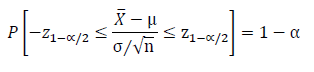
$//<![CDATA[ \begin{array}{l}P\left[ -z_{1-\alpha/2} \leq \frac{\overline{X} - \mu}{\sigma / \sqrt{n}} \leq z_{1-\alpha/2} \right] = 1 - \alpha\end{array} //]]>$

The following equation is then produced after rearranging within the inequality by multiplying all terms by σ/√N:

The population standard deviation in the above equation, σ, is substituted with S, which is the estimate of the standard deviation from the sample of size N, to produce Equation the following equation.

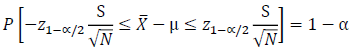
$//<![CDATA[ \begin{array}{l}P\left[ -z_{1-\alpha/2} \frac{\sigma}{\sqrt{N}} \leq \overline{X} - \mu \leq z_{1-\alpha/2} \frac{\sigma}{\sqrt{N}} \right] = 1 - \alpha\end{array} //]]>$

Thus, the resulting expression (above equation) yields a 1-α probability that the sample mean is less than the distance of the estimate is from the true mean (equation below).

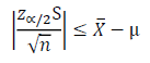
$//<![CDATA[ \begin{array}{l}\left| \frac{z_{\alpha/2} S}{\sqrt{n}} \right| \leq \overline{X} - \mu\end{array} //]]>$

The minimum distance threshold from the true mean can be specified by setting an acceptable value for the error. For this example, the error is _X-μ (above equation). However, the error could alternatively be represented as a percentage of the mean estimate, which would be as follows in the equation below:

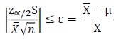
$//<![CDATA[ \begin{array}{l}\left|\frac{\mathrm{z}_{\alpha / 2} \mathrm{~S}}{\bar{X} \sqrt{n}}\right| \leq\varepsilon=\frac{\overline{\mathrm{X}}-\mu}{\overline{\mathrm{X}}}\end{array} //]]>$

Expressing the error as a percentage, allows the calculation to be evaluated regardless of the magnitude of the random variable (equation below).

$//<![CDATA[ \begin{array}{l}\left|\frac{\mathrm{Z}_{\propto / 2} \mathrm{~S}}{\bar{X} \sqrt{n}}\right| \leq \varepsilon\end{array} //]]>$

Since neither the sample mean, X, nor the sample standard deviation, S, known a priori, this equation must be evaluated at the completion of every iteration. Once the equation becomes true, sufficient samples have been made to conclude that the sample mean is within ε distance from the true mean with 1-α confidence.

Empirical Distribution

An empirical distribution is a data collection tool specified by quantile. An empirical distribution consists of cumulative probabilities and their coinciding quantiles. Summary statistics are solved using discrete integration. The quantile function is relatively simple for the empirical distribution. If the random number p matches one of the cumulative probabilities in the data, then the relevant quantile is returned, otherwise we find the interval of cumulative probabilities in which the random number p would lie and linearly interpolate.