Download PDF
Download page New Features.
New Features
- Habitat quality. New features were added that allow users to add, copy, rename, and delete paired data sets known as Habitat Suitability Indices (HSIs). HSIs relate a variable such as water depth or velocity to a measure of habitat quality that ranges from 0 (wholly unsuitable) to 1 (perfectly suitable). HSIs are commonly used in ecological modeling, including model applications for habitat mapping (Figure 1).
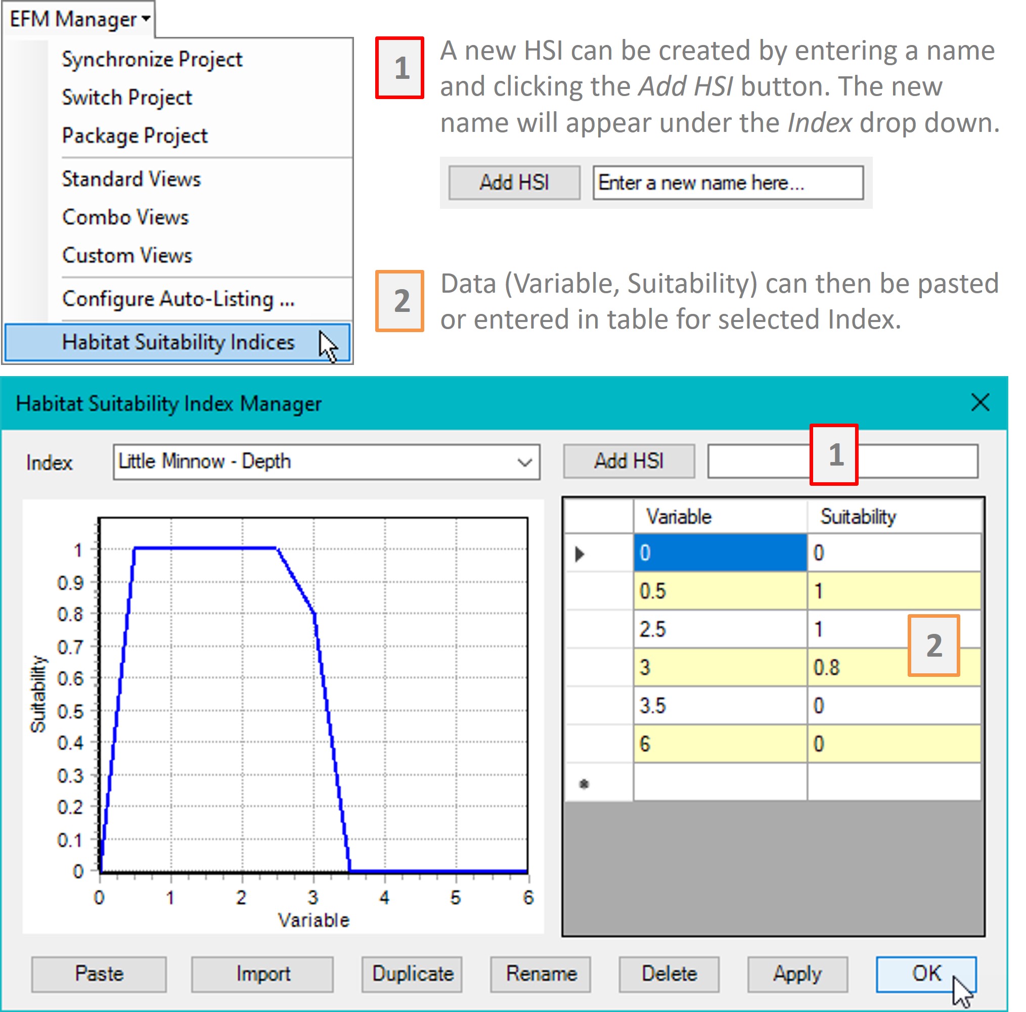
Figure 1. Menu option and interface related to HSIs in GeoEFM.
HSIs are applied via the GeoEFM calculator and batch calculator. HSIs are applied to raster layers. For example, in Figure 2, shows a HSI (Little Minnow – Depth) being applied to a raster of water depths (nat-minnow) to generate a suitability raster (NaMi_Suit_Hab, which is an abbreviated name referring to a raster of suitable habitat for the EFM flow regime “Natural” and the EFM relationship “Little minnow”).
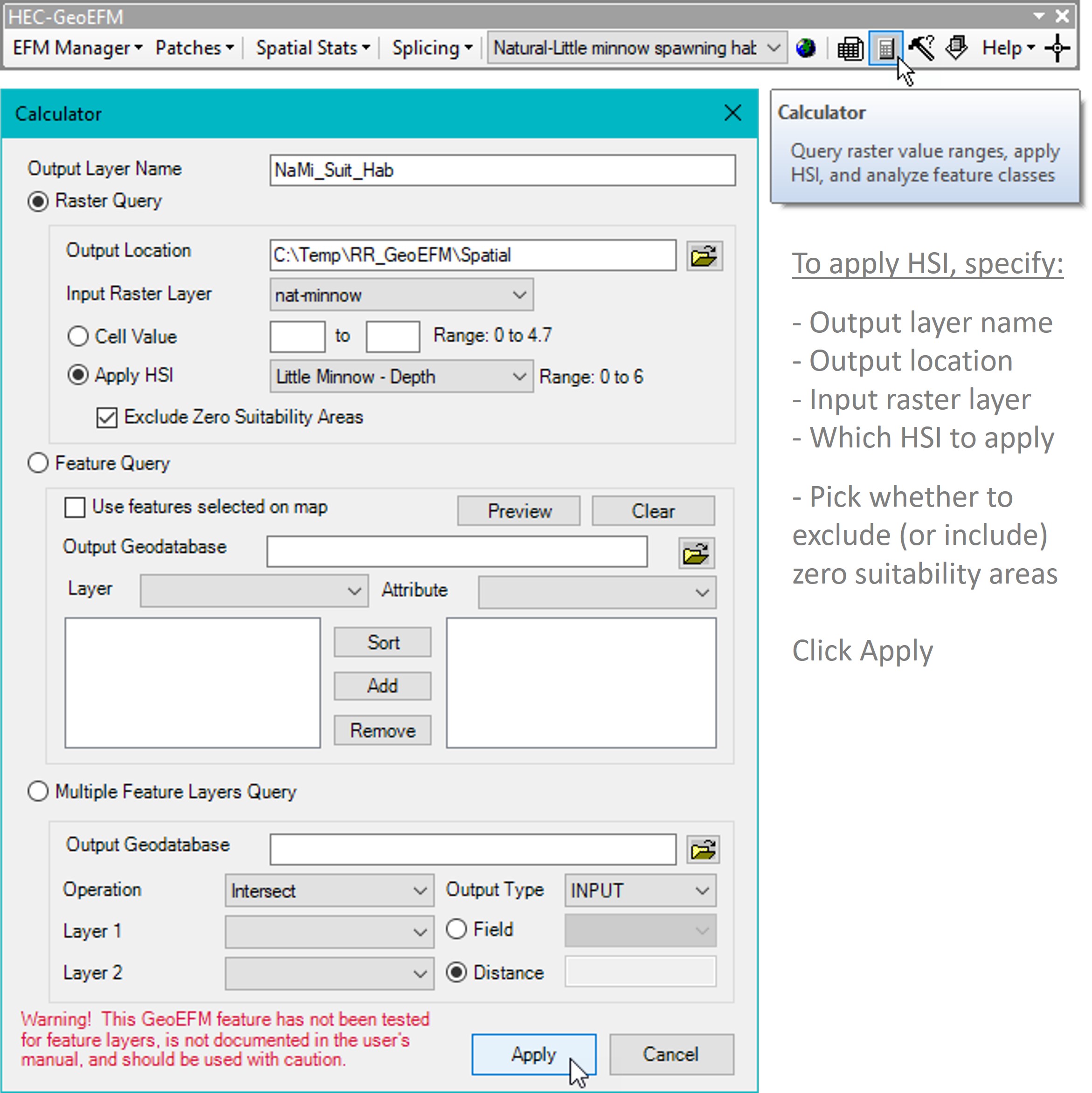
Figure 2. Application of HSI to generate a suitable habitat raster using the GeoEFM calculator.
An option is provided that allows the users to pick whether to exclude (checked) or include (unchecked) zero suitability areas from the output raster (Figure 3).
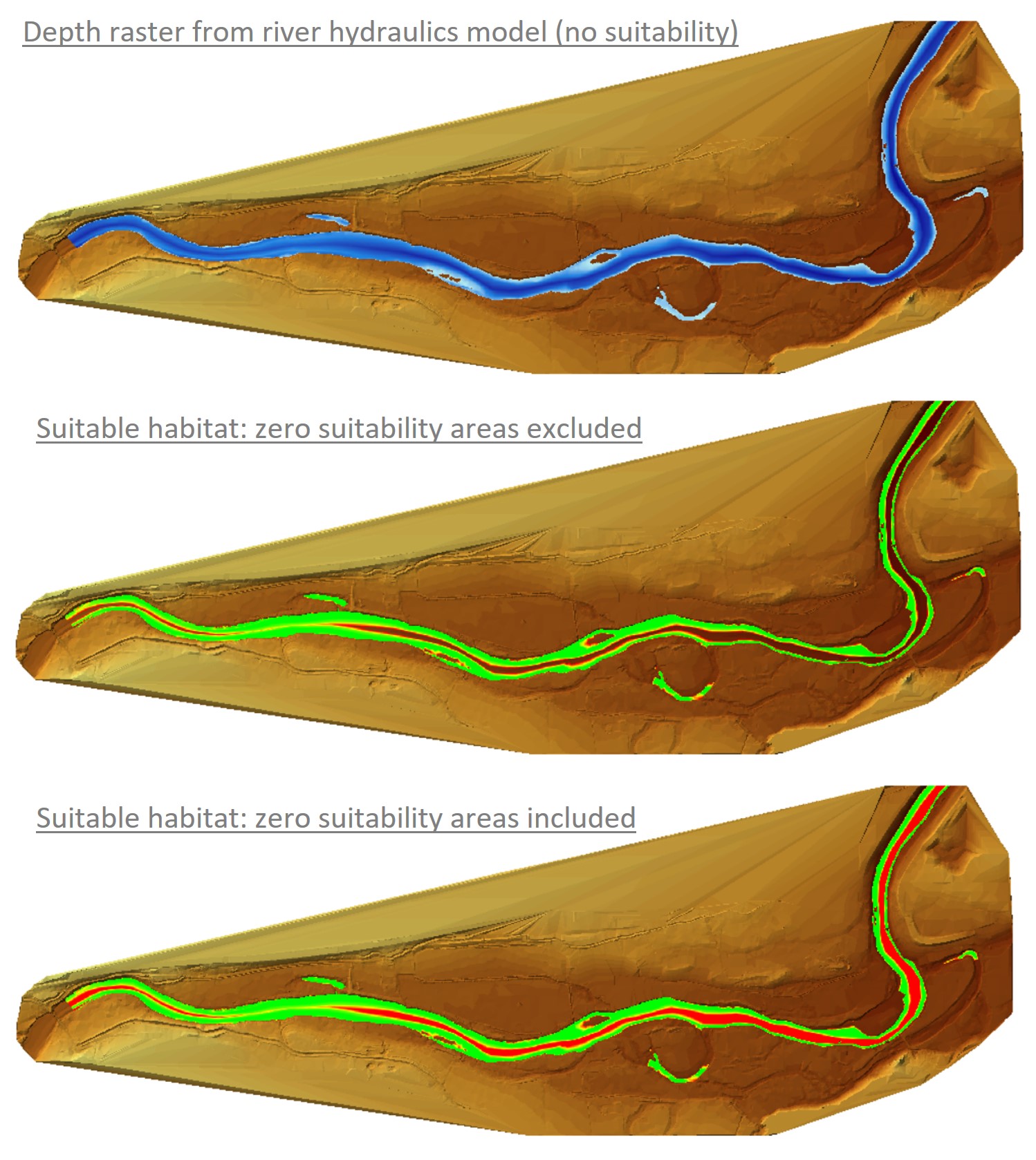
Figure 3. Suitable habitat rasters generated without and with zero suitability areas.
- GeoEFM has two calculators, one that performs single instance queries of spatial layers (Calculator; Figure 2) and one that performs repeating queries of spatial layers (Batch Calculator). In addition to the HSI features described above calculators can also be used to query raster value ranges (Figure 4). It also has several components related to working with feature classes, though those have not been rigorously tested and should be used with caution.
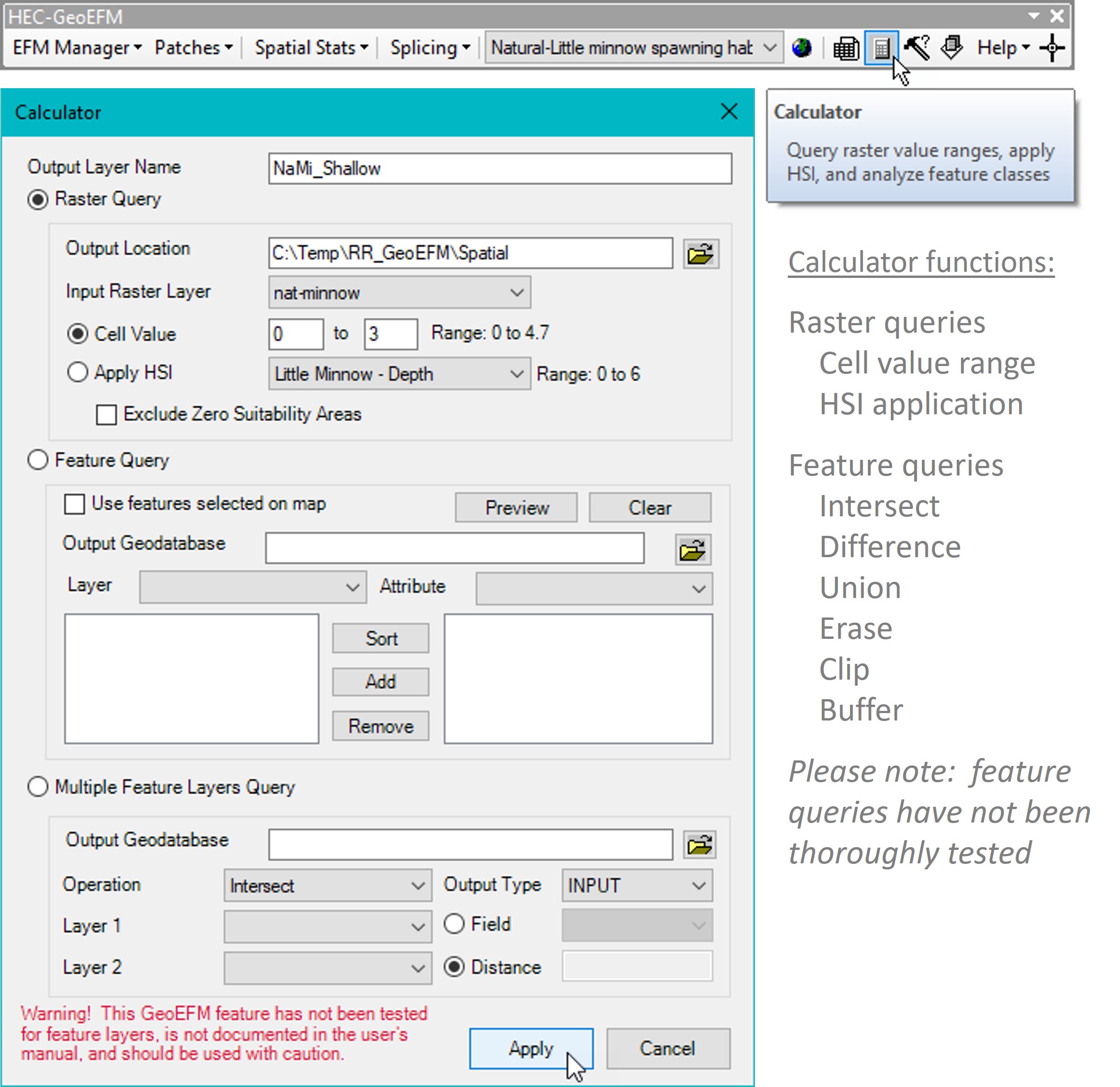
Figure 4. GeoEFM calculator being used to apply a raster cell value range.
Cell value is a simple query that applies a user-defined range to an input raster resulting in an output raster that contains only the cells and corresponding values that are within the range (Figure 5). Ecologically, this is typically used to filter areas that are not relevant to the EFM relationship being considered. In this sense, cell value is similar to the apply HSI option, though cell value does not allow for partial suitability, areas are either in range or dropped from the output layer.
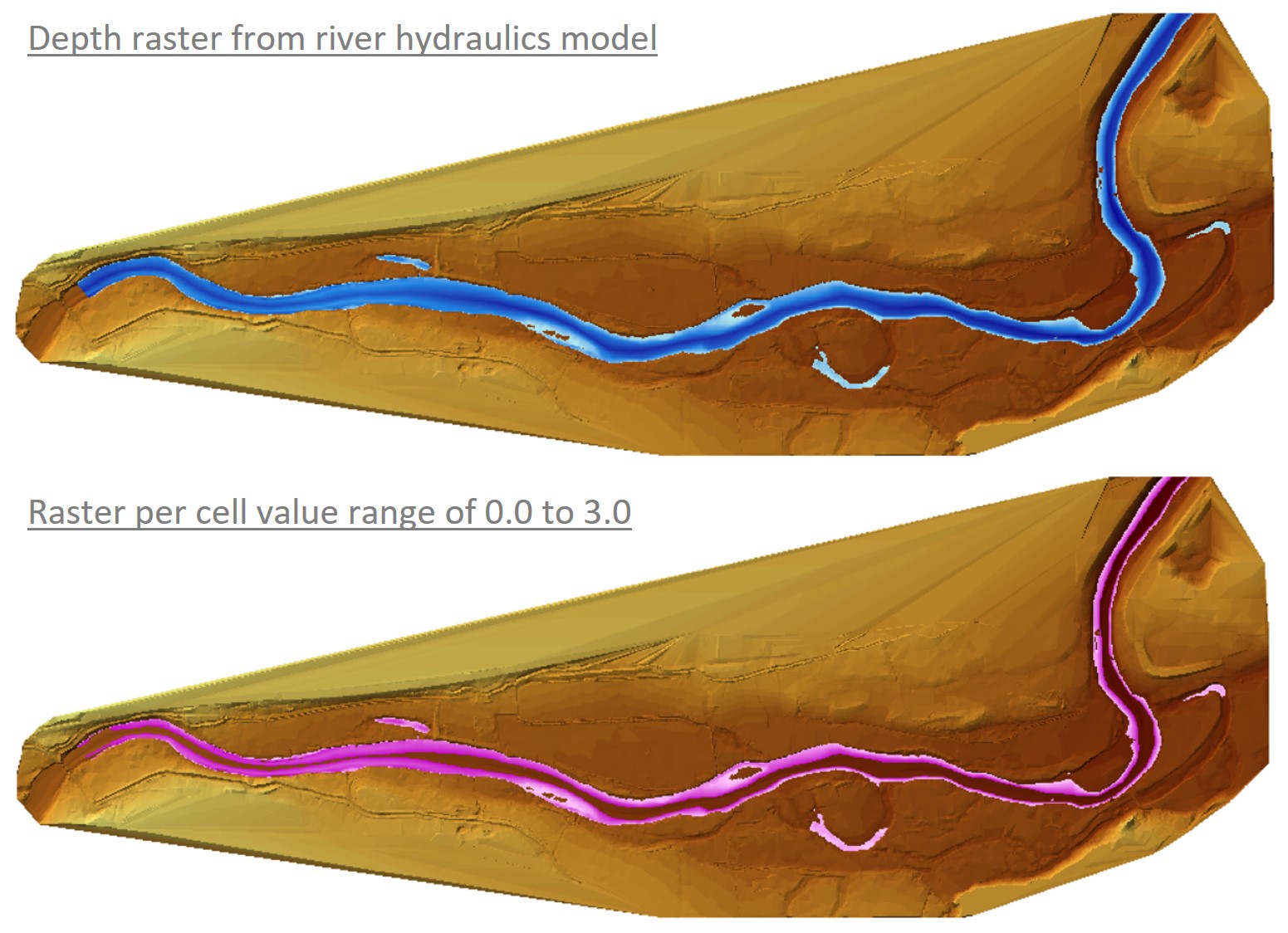
Figure 5. Top image shows a depth raster (blue) from a river hydraulics model. Bottom image show raster of depths from 0.0 to 3.0.
The batch calculator performs a user-defined spatial operation for multiple raster layers. This feature is most commonly used when processing layers for one EFM relationship and many flow regimes. In this case, the same spatial operations, whether cell value or apply HSI, needs to be done for each of the implicated relationship-flow regime pairings (Figure 6).
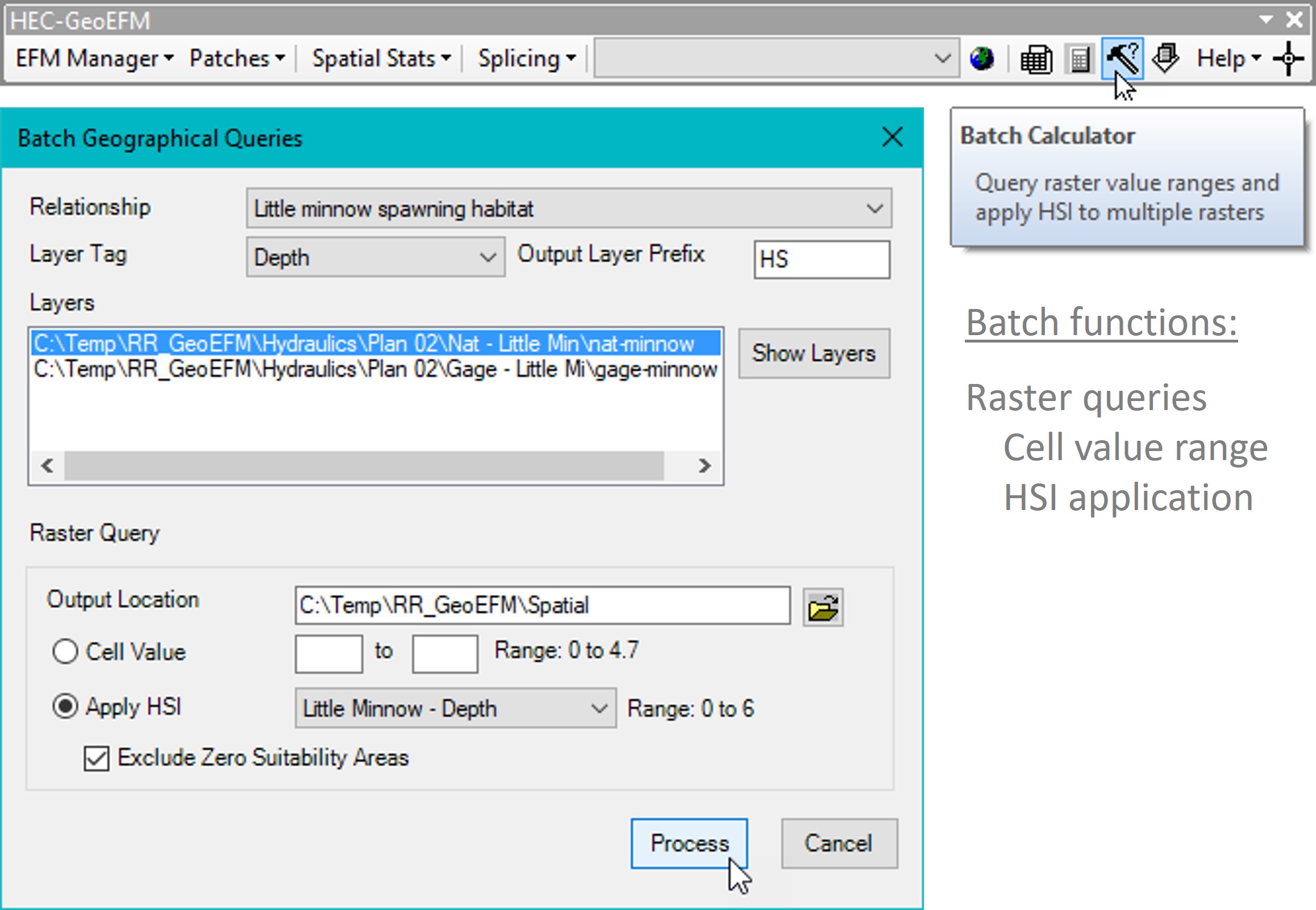
Figure 6. GeoEFM Batch Calculator interface being used to apply a HSI to multiple raster layers.
- Integration of habitat quality with existing GeoEFM tools. GeoEFM’s tabulate and physical connectivity features were expanded to include habitat quality considerations. For example, the GeoEFM tabulate tool was expanded to include an option to tally suitable habitat in addition to total habitat areas (Figure 7).
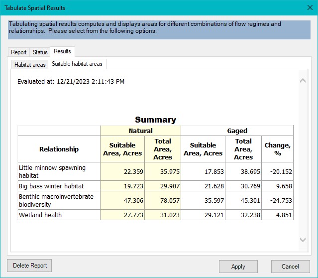
Figure 7. Suitable and total habitat areas for select pairings of flow regimes and relationships.
- Habitat functionality. Ecological concepts like habitat corridors, fragmentation, and functionality can be explored using the GeoEFM patch tool. In version 2.0, two new methods were added to the patch tool, nearest neighbor and buffer. Both methods were adapted from ecological literature related to habitat connectivity. Both methods parse habitat in a raster layer into the unit habitat areas (i.e., patches) that would support individuals or groups of individuals within a population.
Nearest neighbor is most applicable to gregarious communities that are not strongly territorial. Figure 8 shows nearest neighbor patch results for a raster processed with suitabilities. Larger patches occur in the poorest habitat because more total area is required to meet the user-specified area (suitable) required to make a patch.
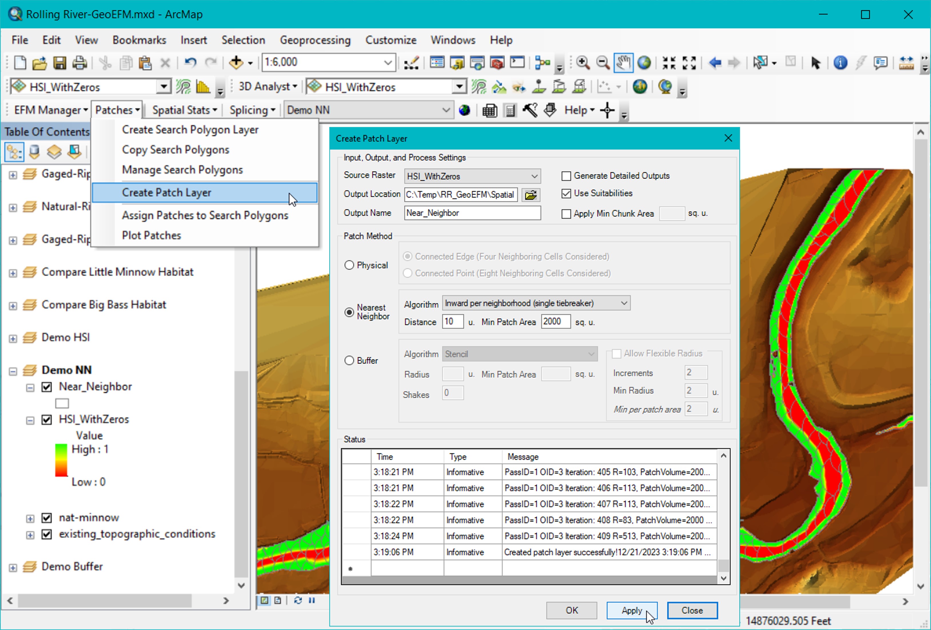
Figure 8. Creating a patch layer using the GeoEFM nearest neighbor method.
Buffer is most applicable to territorial communities that inhabit or utilize or protect an area for one or more of their life stages such as nesting. Figure 9 shows buffer patch results for a raster processed with suitabilities. Patches cut with the larger radius (50 map units) tend to occur in the poorest or sparsest habitat because the larger radius was needed to meet the user-specified area (suitable) required to make a patch.
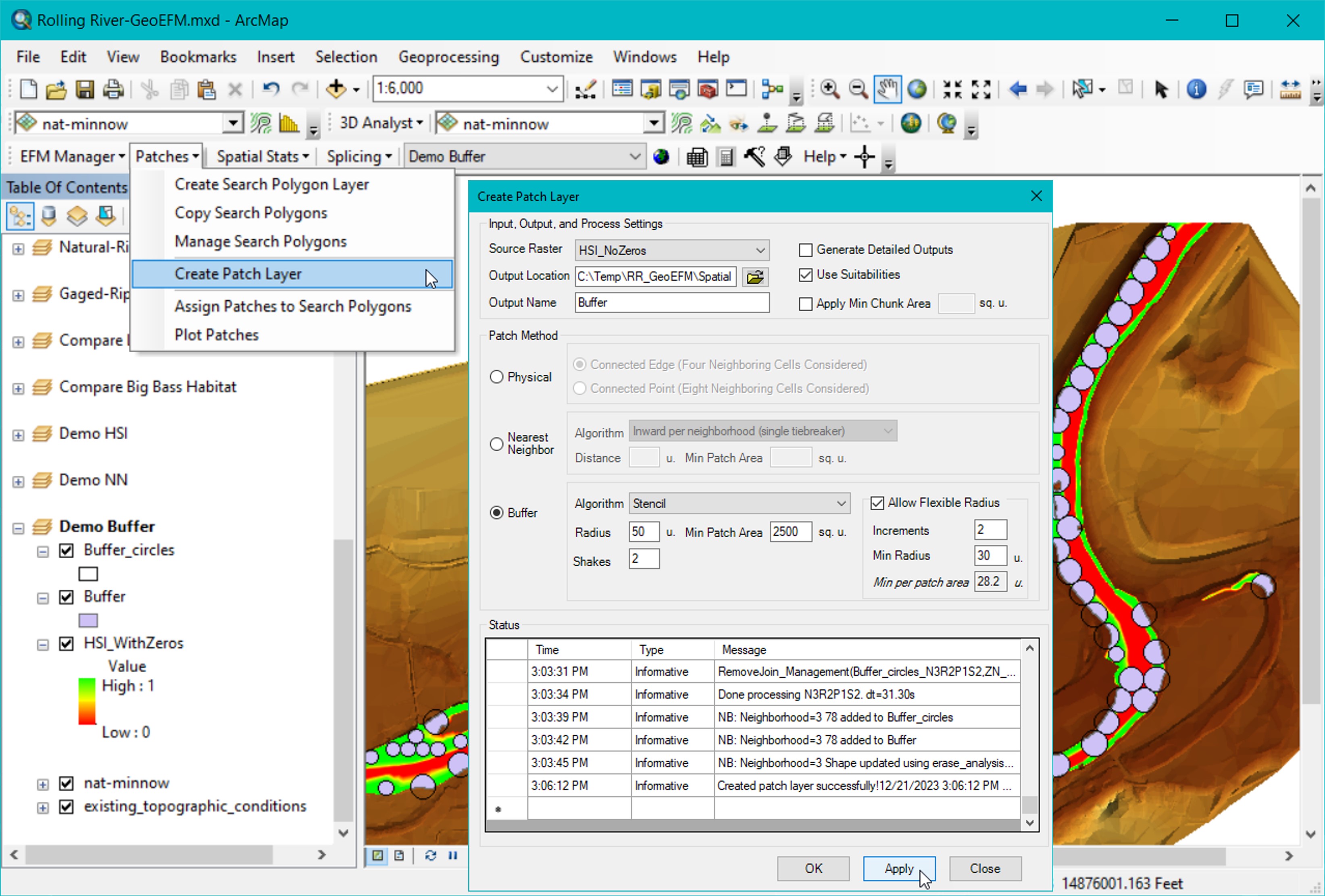
Figure 9. Creating a patch layer using the GeoEFM buffer method.
- Habitat mosaics. New features were added to help create habitat mosaics. For example, these features would allow habitat in a tributary stream and its receiving river to be spliced into a single habitat map. In EFM, the stream and river would be assessed separately for the same relationship because each has a different flow regime. Statistical results would be simulated with a hydraulics model to generate maps for the stream reach and for the river reach. Splicing tools in GeoEFM would assist with merging the two layers spatially to create a single map for that habitat type. The basic process for splicing is to make a splicing configuration and then apply it to a set of layers. There are three types of configurations: Polygon, raster, and hydraulic model (Figure 10).
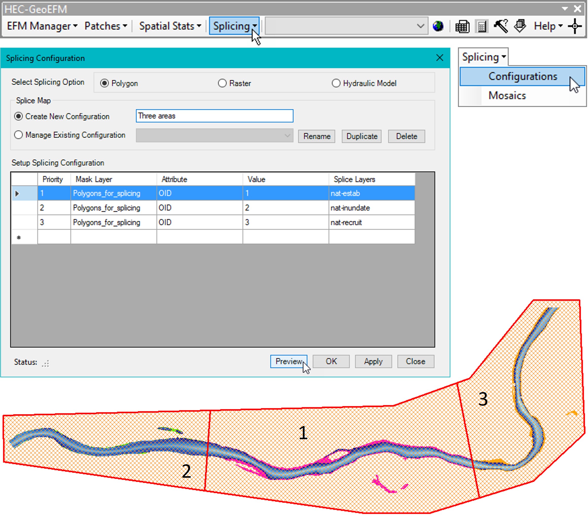
Figure 10. Interface for and preview of a polygon splicing configuration.
Choice of type is controlled by the user via the Select Splicing Option feature. Mosaics made with the polygon option are much like quilts. Polygons are used to define the areas of the quilt and the layers associated with those areas serve as the fabrics that are stitched together to form the mosaic. The raster option uses rasters as both the domain and the areas within that domain to be included in the splice. The hydraulic model option allows mosaics to be assembled based on the layout of 1-dimensional river hydraulics models (Figure 11).
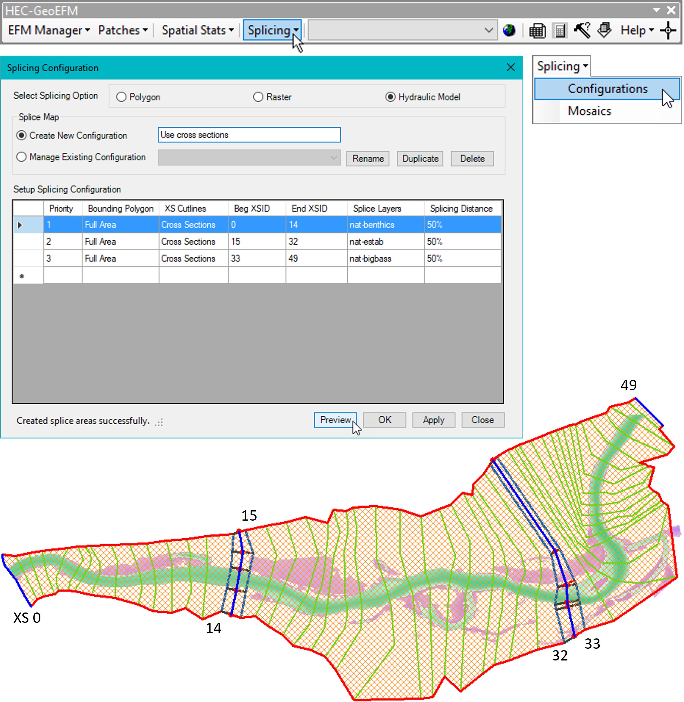
Figure 11. Interface for and preview of a hydraulic model splicing configuration.
The splicing interface executes splices per the use-selected configuration. Options are offered for handling raster cell offsets and overlaps. The mosaic generated is a raster and is displayed in the current view (Figure 12).
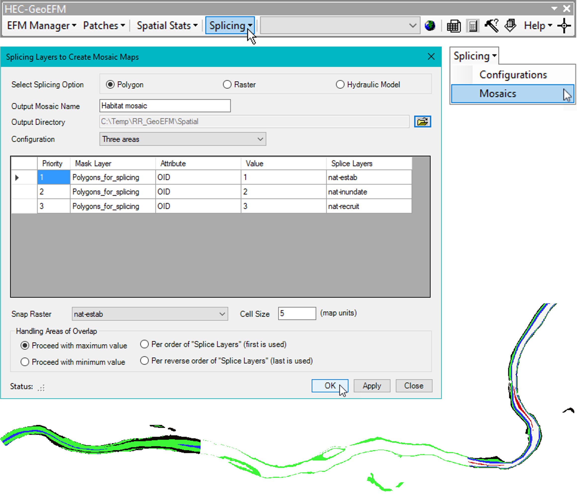
Figure 12. The splicing interface allows users to select and apply combinations of configuration, snap raster, and overlap option to create raster mosaics.
- Spatial statistics. New features were added that allow users to display statistical results spatially. This is a different workflow than using a river hydraulics model to generate spatial layers based on EFM results. Instead, statistical results (or derivations based on those results) are associated with locations and then plotted. Information for plotting are stored in three basic data tables: Locations, relationships, and datasets (Figure 13).
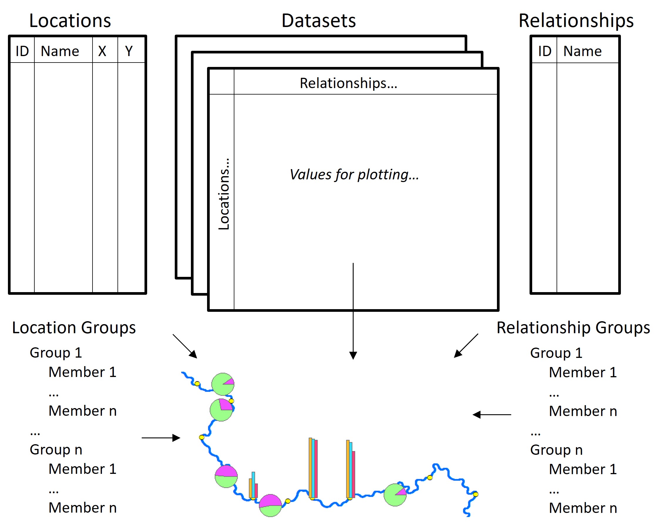
Figure 13. Process and data tables related to GeoEFM mapping of spatial statistics.
After the locations, relationships, and dataset tables are populated, data values may be viewed spatially. Three chart types are available: bar, pie, and stacked. Colors can be adjusted by switching the start and end of ramp colors. When the plot button is clicked, an output layer will be displayed as part of the active data frame (Figure 14). Output layer names do not need to be unique, though duplicate names will replace the existing output layer.
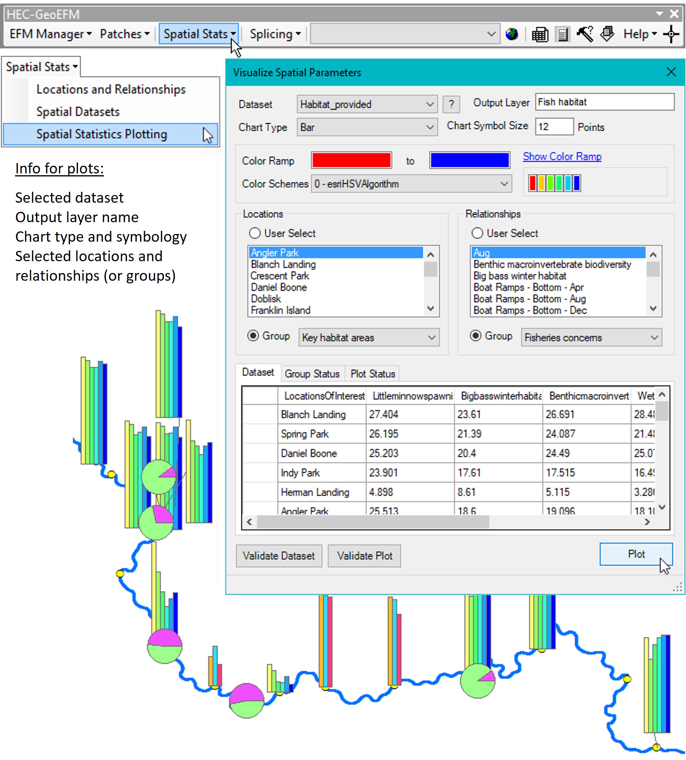
Figure 14. Spatial statistics are plotted via the Visualize Spatial Parameters interface.
Configure Auto-Listing. The configure auto-listing interface allows users to select whether GeoEFM generated layers are automatically associated with their corresponding views when those layers are created (Figure 15). This is a handy time-saving option, especially when working with habitat suitability indices, habitat splicing, and habitat functionality. Each of those GeoEFM features is capable of producing many output layers. The top checkbox option is a master on/off switch. When deselected, auto-listing is off regardless of the other checkbox settings.
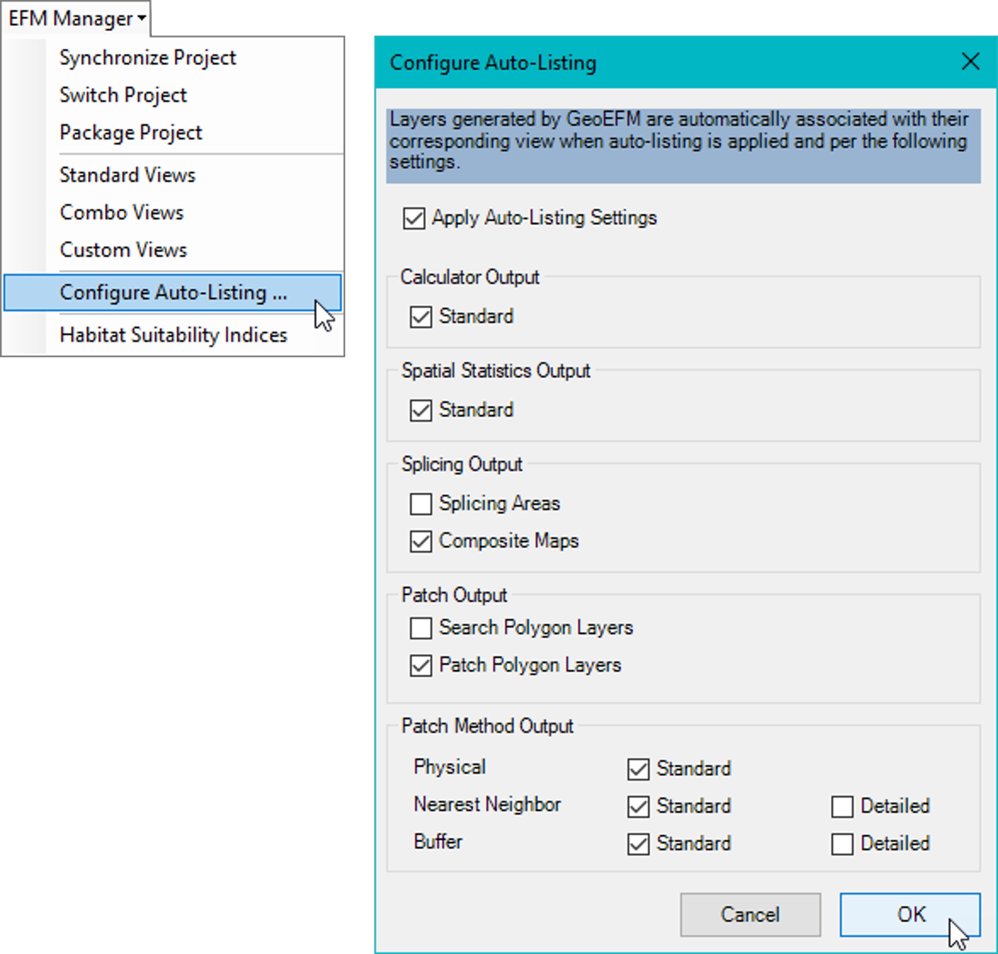
Figure 15. Auto-Listing supports management of layers generated by GeoEFM.