Download PDF
Download page Applying the Recession Baseflow Method.
Applying the Recession Baseflow Method
Last Modified: 2025-01-29 17:48:26.904
Overview
In this tutorial you will apply the HEC-HMS Recession baseflow method to a modeling application. Initial parameter estimates will be determined, and the model will be calibrated through trial and error.
Software Version
HEC-HMS version 4.13-beta.4 was used to create this example. You can open the example project with HEC-HMS 4.13 or a newer version.
Project Files
Download the Initial project files here:
Note: The initial project file is the same for the Constant Monthly, Recession, and Linear Reservoir Baseflow tutorials. If you are completing all three tutorials, the files only need to be downloaded once.
Initial Parameter Estimates
- Open the Punxsutawney project and then open the Mahoning Creek Recession Basin Model.
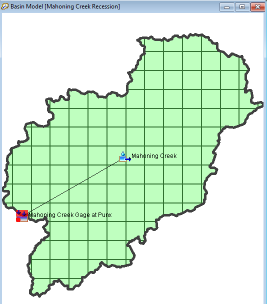
- Select the Sept2018_Recession simulation run from the Compute toolbar,
 . Press the Compute All Elements button,
  , to run the simulation.
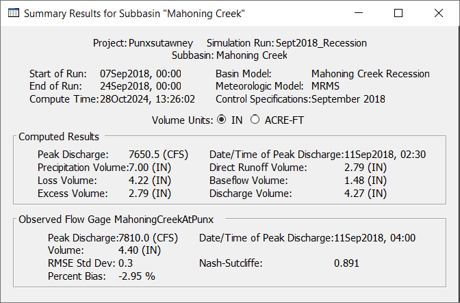
 - View the result graph and summary table for the Mahoning Creek subbasin element. Notice the computed flow does a good job matching the peak observed flow, but the interflow and baseflow portions of the computed hydrograph do not match observed flow. The summary table shows a large difference in observed and computed runoff volume (4.40 inches vs. 2.79 inches). Leave the summary table and plot open so you can see results change as you add baseflow and modify baseflow parameters.


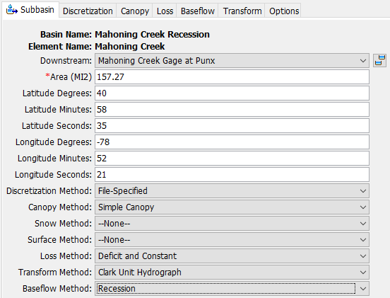
- Open the Component Editor for the Mahoning Creek subbasin element. Change the Baseflow Method from None to Recession.
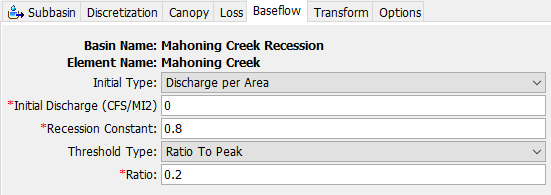
- Go to the Baseflow tab to enter Recession parameters. Change the Initial Type to Discharge per Area. Enter an Initial Discharge of 0 CFS/MI2. Enter 0.8 as the Recession Constant. Enter a Ratio to Peak value of 0.2.
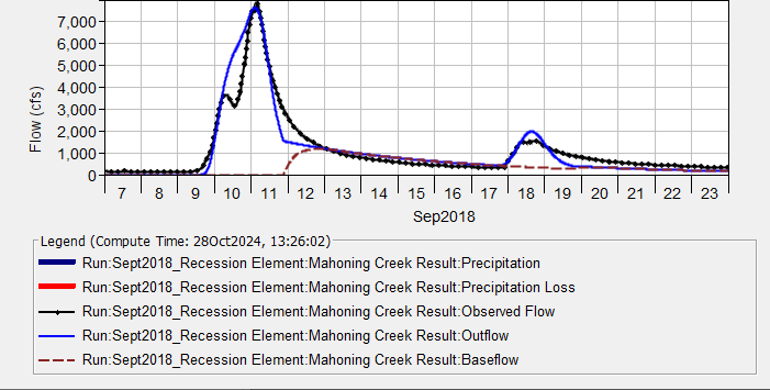
- Re-run the simulation and look at the results plot and summary table. Notice baseflow in the plot and how the addition of baseflow to direct runoff results in an increase in the simulated flow. The total runoff volume increased as well. The direct runoff is 2.79 inches and the baseflow is 1.48 inches.
Calibrate the Model
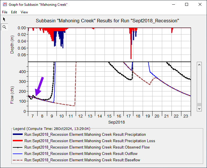
- The easiest baseflow parameter modification to make is to set the initial baseflow at the beginning of the simulation so results match observed flow. If you zoom into the plot, you will see the observed flow value is approximately 160 cfs at 00:00 on September 7, 2018. The drainage area for the subbasin is 157.27 square miles; therefore, the initial baseflow can be set by dividing 160 cfs by 157.27 square miles, which is approximately 1 CFS/MI2. Change the Initial Discharge from 0 to 1 CFS/MI2. Re-run the simulation. You should notice a close match in observed and computed flow at the beginning of the simulation.
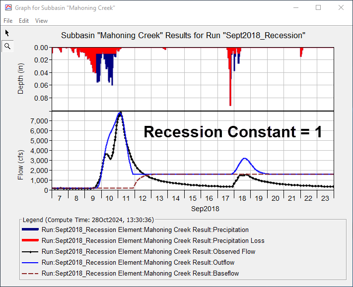
- The Recession Constant parameter impacts the slope of the baseflow hydrograph. Change the Recession Constant from 0.8 to 1.0 and rerun the simulation. You will see a constant/flat baseflow response, there is no recession when the Recession Constant is 1.0. Notice the loss and baseflow volumes in the summary table. The baseflow volume, 4.55 inches, exceeds the loss volume, 4.22 inches.
Change the Recession Constant to 0.4 and rerun the simulation. Notice the baseflow response now simulates a recession curve (there is a decreasing flow rate). A value of 0.4 is too low, the recession is too fast, but do not change the Recession Constant as we look at the Ratio to Peak in the next step.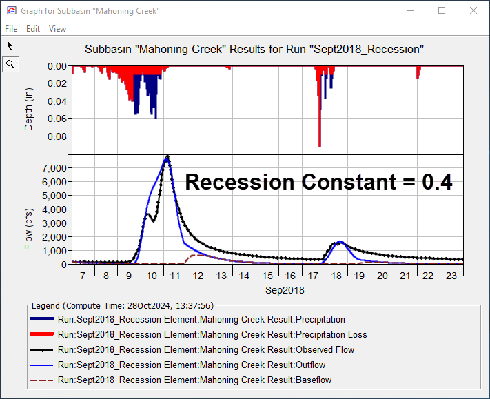
- The Ratio to Peak parameter determines when the baseflow recession curve is added to the total runoff hydrograph. If the peak flow rate is 100 cfs and the ratio to peak is 0.2, then the recession baseflow curve will turn on when the hydrograph reaches 20 cfs (0.2 * 100 cfs). In our September 2018 simulation, the peak flow is approximately 7800 cfs on September 11. Looking at the observed flow hydrograph, it looks like the inflection point in the recession limb occurs around 3000 cfs (at this point, interflow/baseflow become the major contributors to total runoff and not direct runoff). Dividing 3000 cfs by 7800 cfs equals approximately 0.38. Change the Ratio to Peak parameter to 0.38 and rerun the simulation. You should see the baseflow recession curve "turns on" earlier on the hydrograph recession.
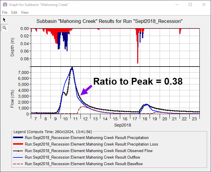
- Continue adjusting the Recession Constant and Ratio to Peak parameters to calibrate the model. Record your Nash-Sutcliffe score as you adjust model parameters.
Project Files
Download the Final project files here:
Note: The final project file is the same for the Constant Monthly, Recession, and Linear Reservoir Baseflow tutorials. If you are completing all three tutorials, the files only need to be downloaded once.
Questions:
Question 1: Can the Recession baseflow method model both interflow and baseflow?
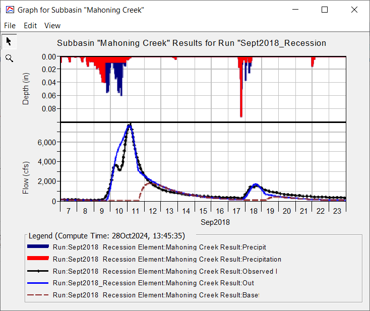
No, the recession method is limited to modeling either interflow or baseflow because you can only define one recession constant and ratio to peak parameters. You can choose to model interflow or baseflow, or attempt to approximate both. The following figure shows results from the recession baseflow method in the example application. Notice how the recession curve is not steep enough for interflow and is too steep for the slower responding baseflow. We would need two sets of recession parameters to model interflow from September 11 through the September 13 and then baseflow from the September 13 through the September 17.
Question 2: Does the Recession baseflow method conserve volume? What information should you always look for when using the Recession baseflow method.
No, the recession baseflow method does not conserve volume. It is possible for the model to generate more runoff volume than precipitation volume when using the recession method. This is why it is important to look at the Subbasin Summary Table and make sure the precipitation, loss, direct runoff, baseflow, and total discharge volumes are reasonable/appropriate. An important consideration is that the same recession baseflow parameters are not transferable to a range of flood events, from mild to extreme. For example, a ratio to peak parameter that might be appropriate for a minor flood event will not be appropriate for a larger event as it will result in too much baseflow volume (0.2 * 1,000 cfs vs. 0.2 * 100,000 cfs results in different recession curves and baseflow volumes).
Question 3: What were your final Recession baseflow parameters? What was the Nash-Sutcliffe score for the calibrated model?
The final Recession Constant was 0.6 and the final Ratio to Peak was 0.4. The Nash-Sutcliffe score was 0.908 with the final recession baseflow parameters.

This tutorial concludes the Applying Baseflow Methods in HEC-HMS tutorial group.
