Download PDF
Download page Task 2: Debris Yield Modeling without Debris Basin (with New Debris Volume Conversion to Mass Unit Weight/Density).
Task 2: Debris Yield Modeling without Debris Basin (with New Debris Volume Conversion to Mass Unit Weight/Density)
Last Modified: 2023-10-24 06:40:07.931
Overview
This workshop illustrates four methods for estimating debris yields using HEC-HMS. In the first workshop, the computed debris yield was based on initial parameter estimates, and debris yields were estimated for only a single storm event. Debris basins periodically need to be cleaned out and volume measurements can be taken based on the number of truckloads needed to empty the basin. From November 2002 to the beginning of April 2003, the debris yield measured at Brand Canyon debris basin amounted to 81,358 m3. The total sediment volume is one piece of information that can be used for debris volume calibration.
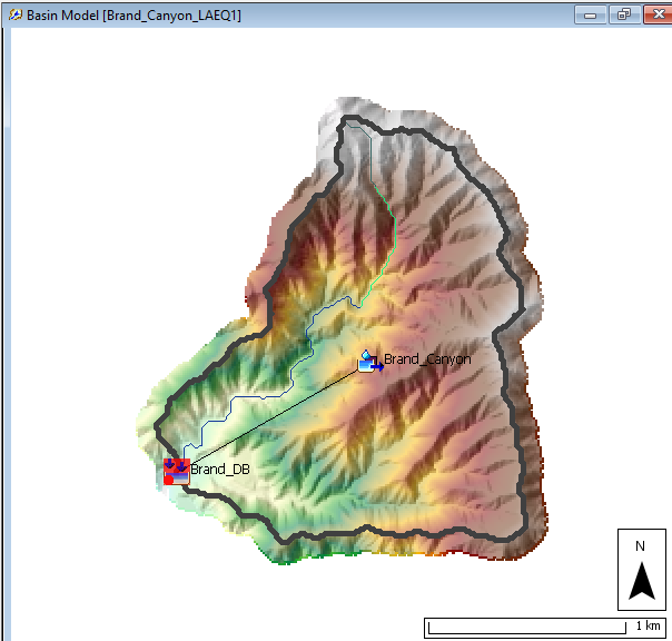
An HEC-HMS model for Brand Canyon watershed has been prepared for you. A Digital Elevation Model was added to the project and used to delineate the Brand Canyon watershed in HEC-HMS. Watershed delineations can easily be performed in HEC-HMS given a projected terrain file. HEC-HMS can also extract watershed characteristics after a basin is delineated. The following HEC-HMS tutorials and guides provides more information on watershed delineation with HEC-HMS.
Data
Download the initial project files here: Debris Yield Workshop wo DB - Existing Model_Initial.zip
Set up Debris Yield Model for LA Debris Yield Equation 1
- Launch HEC-HMS version 4.12 beta 1 or greater and open the project named Brand_Debris_Basin.hms. Select the Basin Models folder to see all the basin models in this project. You should notice a separate basin model for each debris yield method (LAEQ1, MSDPM, USGS_EA, and USGS_LT). We will first look at the Brand_Canyon_LAEQ1 Basin Model.
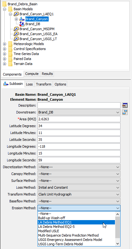
- Select the Brand_Canyon_LAEQ1 Basin Model.
- Select the Brand_Canyon subbasin element.
- On the Subbasin tab, change the Erosion Method to LA Debris Method EQ1.
- Calculate Relief Ratio using the characteristics of subbasin element by selecting Parameters | Characteristics | Subbasin. Select Continue if a message stating "No sink fill raster was found for this basin" appears.
- Convert Relief Ratio from dimensionless units to M/KM by multiplying 1000
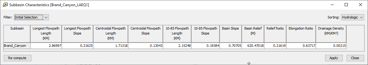

Subbasin Characteristics can only be computed if the watershed was delineated in HEC-HMS. Subbasin characteristics cannot be extracted without the terrain information.
- Convert Relief Ratio from dimensionless units to M/KM by multiplying 1000
- Select the Erosion Tab.
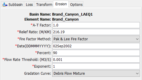
- Populate the initial subbasin parameters based on the given field data shown below. Erosion parameters are described in the User's manual.
- A-T Factor: 1.0 (Set "1" as a default value because the Brand debris basin is located in Southern California).
- Relief Ratio (M/KM): 216.19 (from Subbasin Characteristics).
- Fire Factor Method: Pak & Lee Fire Factor.
- Date (DDMMMYYYY): 02Sep2002 (from Fire record).
- Percent: 90 (from Fire Map).
- Flow Rate Threshold (M3/S): 0.001 (Calibration Factor: This value will be calibrated later with the debris yield measured data).
- Exponent: 1 (Use the Default Value. This controls the shape of the sedigraph).
- Gradation Curve: Debris Flow Mixture (from soil samples at the debris basin location).
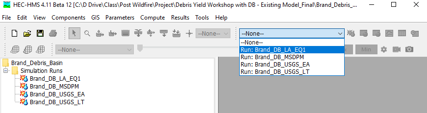
- Run Brand_DB_LA_EQ1 by selecting Run: Brand_DB_LA_EQ1 then click the raindrop icon
 .
.
- Navigate to the Results tab to review your sediment results.
- The Sediment Load and Sediment Volume graphs show multiple debris yield events over the course of the simulation period.

- The Sediment Load and Sediment Volume graphs show multiple debris yield events over the course of the simulation period.
- Now that you have your initial debris yield results, we can compare the computed volume against the measured volume. HEC-HMS provides multiple ways to view sediment results. One way is to look at the results through HEC-DSS. We will extract from the DSS outputs the total sediment load for each grain size.
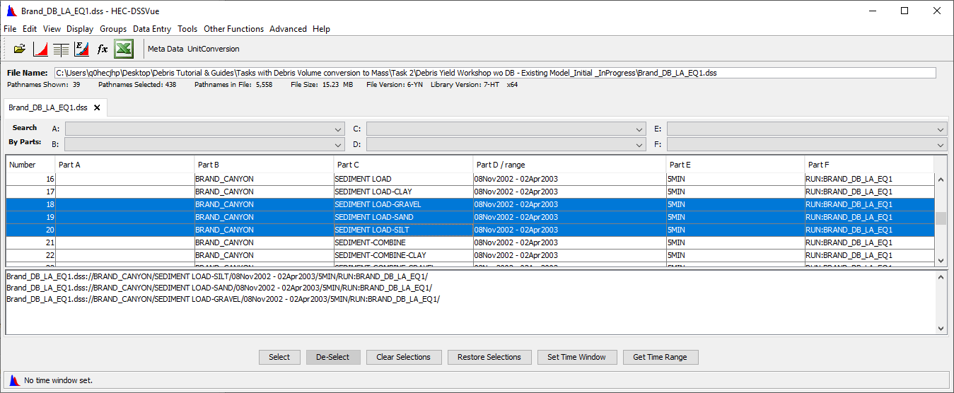
- Go to your project folder and open the output DSS file (Brand_DB_LA_EQ1.dss) for LA EQ1 simulation.
- Double-Click to select the sediment load results for Silt, Sand, and Gravel as shown below.
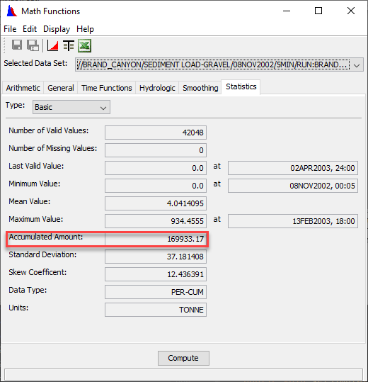
- Click on Tools | Math Functions.
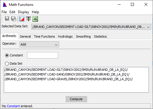
- Click on the Statistics tab then read Accumulated Amount for three grain sizes (silt, sand, and gravel) by changing Selected Data Set. The reported values are in units of tonne.
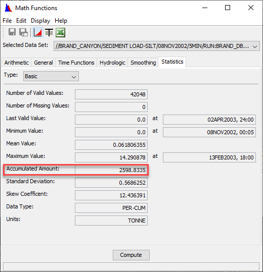

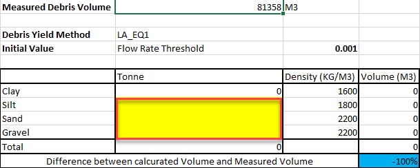
- An excel spreadsheet named Measured Data.xlsx has been prepared for you which can be found in the project folder: Debris Yield Workshop wo DB - Existing Model_Initial\previously_created_data. Select the Initial Results tab. The table calculates the sediment volume given the weight (tonne) and density (kg/m^3) of the sediment. The distribution of silt, sand, and gravel were computed for you based on the gradation curve you initially defined.
Add your accumulated debris amounts (TONNE) to this spreadsheet for each grain size (silt, sand, and gravel) and compare with the measured volume of 81,358 M3.
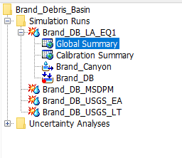
Calibrate the Flow Rate Threshold value by minimizing the difference between your calculated debris volume and measure debris volume. Since the total sediment volume is what is being compared, head back to the Results tab in HEC-HMS and select the Global Summary Table. The Global Summary table provides the combined Sediment Volume and Sediment Load.
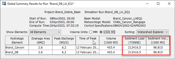
- Change the Flow Rate threshold value and compare the total Sediment Volume against the measured volume. The units are shown in thousand cubic meters.
Once you have selected a threshold, head over to the Measured Data.xlsx spreadsheet and tab over to the Calibration Results. Enter your final values.
Question 1: What is your final value for the Flow Rate Threshold and percentage difference?
Answers will vary. Using a Flow Rate Threshold of 1.7 M3/S the total volume was computed as 76,756 m^3. The Percentage Difference was computed as -6%
Question 2: What is happening when you adjust the flow threshold value?
The flow threshold parameter defines when an "event" has occurred. By increasing the threshold, less debris generating events are occurring. For the debris equation to be used in a continuous model, debris generating events need to be defined.
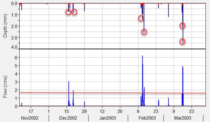
In the graph above, a threshold value of 1.7 m^3/s would suggest 6 debris generating events had occurred within the 5 month window. This means the debris equation was applied for the period when the flow event exceeded the threshold value. For LA Equation 1, the maximum 1-hour rainfall was extracted during the period when the flow threshold was exceeded.
The defined events are also used for the Pak & Lee Fire Factor method and the flow threshold is used as a surrogate to define the number of antecedent effective rainfall events. The Fire Factor decreases as more "events" occur.
Question 3: What assumptions are we making about the simulated water flow?
We assume the flow value determines when there is a debris flow even though the debris equation is computed using maximum rainfall intensity. The simulated flow is also not calibrated. Adjusting parameters that affect the peak flow value, such as constant loss rate, will change the debris yield.
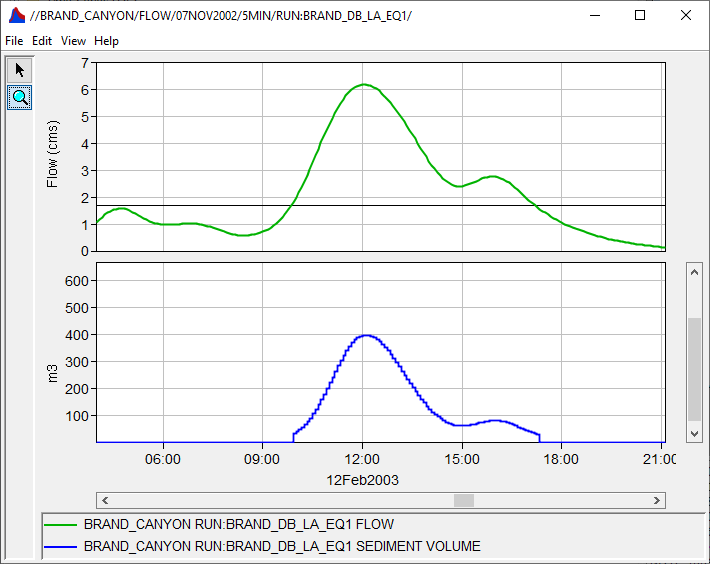
Question 4: What happens when you change the exponent parameter value?
The exponent changes the shape of the sedigraph while preserving the total volume. A value of 1 keeps the sedigraph shape the same as the outflow hydrograph. The sedigraph has a peak volume of around 400 m^3.
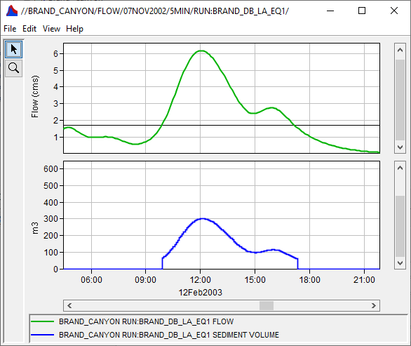
An exponent value of 0.2 flattens the sedigraph as shown in the graph below. The sedigraph volume peak is reduced to around 300 m^3. Note the peak timing of the sedigraph does not change with adjustments to the exponent value.
Set up Debris Yield methods for MSPDM, USGS EA, and USGS LT
- Once you have calibrated your Flow Rate Threshold, perform the calibration to the other debris yield methods (MSDPM, USGS-EA, and USGS-LT).
- Initial parameters for USGS EA and USGS LT can be assigned using the same information provided. The USGS EA and LT methods require the Burn Area parameter in km^2 or mi^2. Multiply the drainage area by the burn area percentage.
- The Flow Rate Threshold will likely be the sensitive parameter for calibrating. Focus on adjusting this parameter.
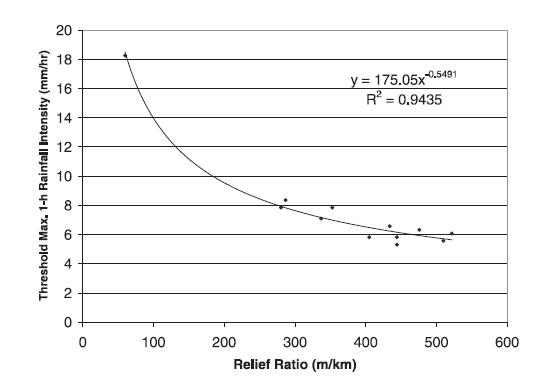
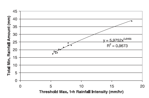
- For the Multi-Sequence Debris Prediction Method, the Max 1-hour Rainfall Intensity and the Total Min Rainfall Amount can be initially approximated using the figures below. This regression was estimated for Southern California basins. The Max 1-hour Rainfall Intensity and the Total Min Rainfall Amount are parameters that trigger when there is enough energy for the debris flow to make it out to the outlet. Both values need to be satisfied in order for debris flow to occur. In addition to the Flow Rate Threshold, you will likely need to adjust these parameters for calibration.
- Initial parameters for USGS EA and USGS LT can be assigned using the same information provided. The USGS EA and LT methods require the Burn Area parameter in km^2 or mi^2. Multiply the drainage area by the burn area percentage.
Question 5: Which method would you choose to use?
Open for discussion
Question 6: Assume you discovered the debris yield collected at the debris basin was generated from a single storm event. How would you change your modeling?
The modeling would be an event based model and the time window can be shortened to the storm event that generated the debris yield. Based on the results from Task 1, the debris yield equations would all underestimate the debris yield. Look closer at parameters that potentially could be uncertain, such as the burn percent or at the rain gage. You can review the burn percent map or measured rainfall to determine if the computed values are representative of the basin location. Spatial data such as gridded rainfall from radar can be looked at since intense rainfall is commonly missed by point rain gages.