Download PDF
Download page Task 4: Debris Flow Modeling using Debris Channel Routing Method.
Task 4: Debris Flow Modeling using Debris Channel Routing Method
Overview
This workshop illustrates debris channel routing methods within HEC-HMS. This workshop focuses on using an existing HEC-HMS model and modifying the methods for a debris flow simulation through the channel element. The HEC-HMS model must be reviewed to understand assumptions made when the model was developed. It is also important to look over the calibration results and assess whether the computed simulation does a good job at replicating measured accumulated debris yield volume (based on the debris basin clean-out records). You may need to make additional adjustments to parameters based on your assessment. In this workshop, you will summarize the model parameters in the existing HEC-HMS model and choose appropriate input parameters for the Deer Creek Debris Basin watershed.
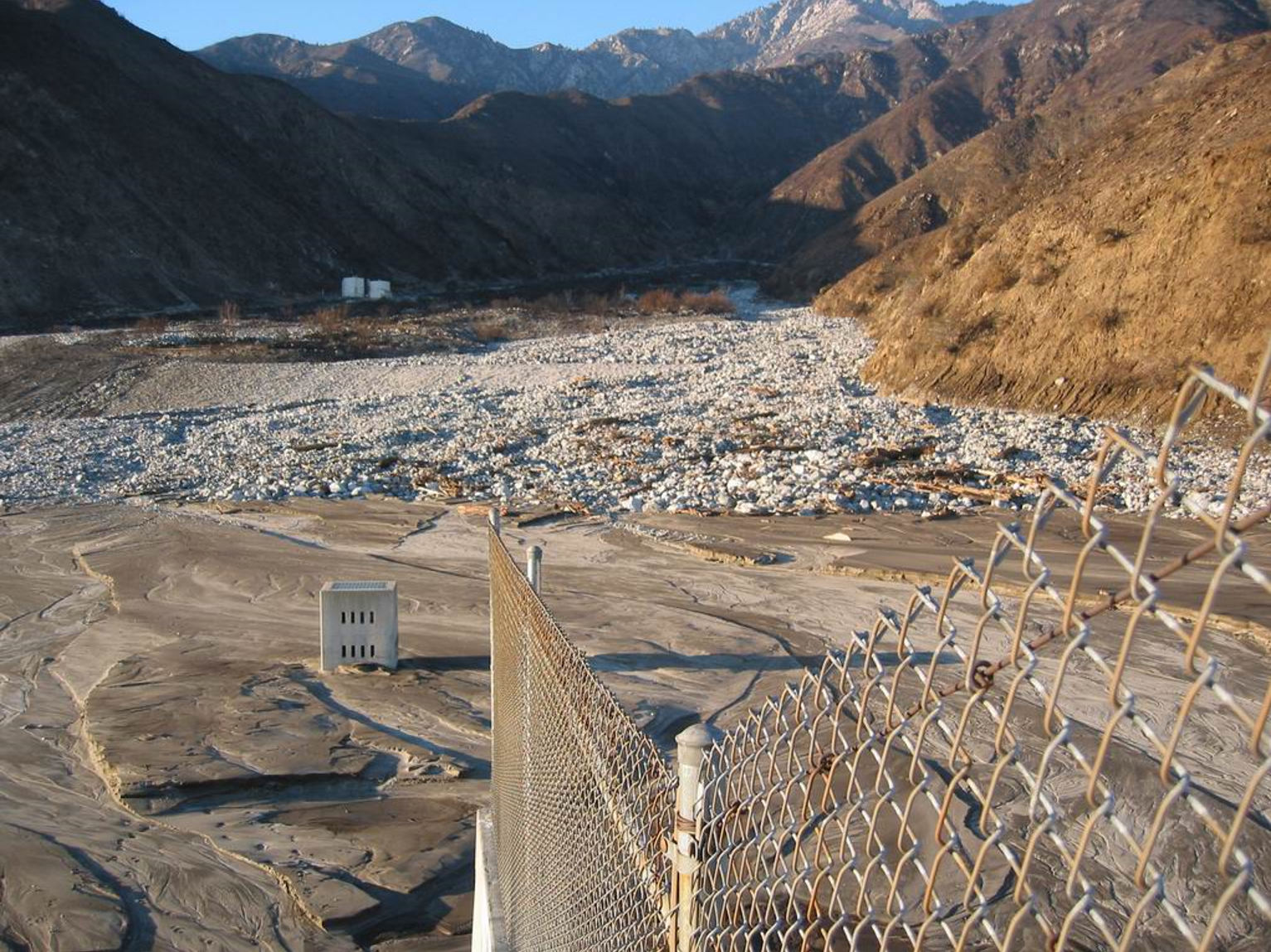
On October and November, 2003, the Padua Fire, Grand Prix Fire, and Old Fire in the San Gabriel Mountains and San Bernardino Mountains burned nearly 36,826 hectares including the watershed of Deer Creek Debris Basin. Precipitation data were collected from three gages [Demens Creek Debris Basin (DCDB), Mt. Baldy (MTBY), and San Antonia Dam (SNTO)], located in the vicinity of the Grand Prix Fire area. After analyzing the data, the MTBY gage was deemed the most reliable due to its accurate rainfall measurements and its proximity to the average elevation of the affected watershed. The debris yield was measured to be 120,112 m3 for the Deer Creek debris basin. The Grand Prix Fire burned the watershed of Deer Creek debris basin completely, as reported by Pak and Lee in 2012.
Data
Download the initial model files here - Deer_Ck_DB_SDR_M_Initial.zip
Review the Model
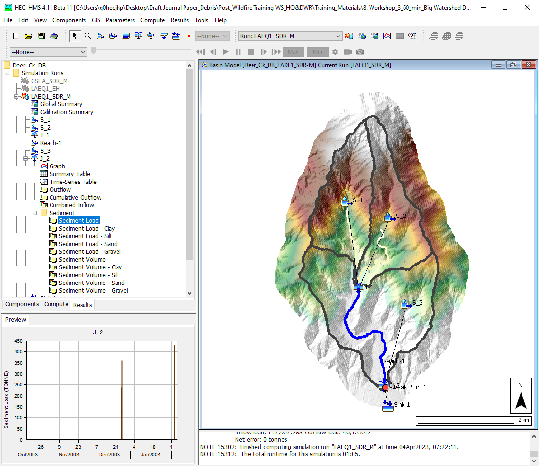
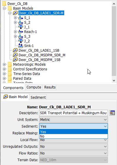
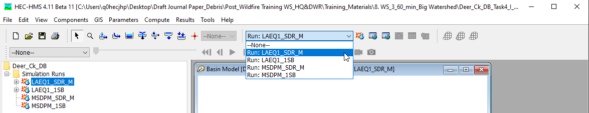
- Launch HEC-HMS version 4.12 beta 1 or newer and open the project by selecting File | Open | Browse. Select the project named Deer_Ck_DB.hms. Select the Basin Models folder to see all the basin models in this project. You should notice a separate basin model for each debris yield method. We will first look at the Deer_Ck_DB_LADE1_SDR-M Basin Model (using LA Debris EQ 1 and SDR + Muskingum methods with 3-subbasin).
- Select the Deer_Ck_DB_LADE1_SDR-M Basin Model.
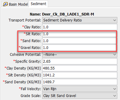
- Select Yes for the Sediment option.
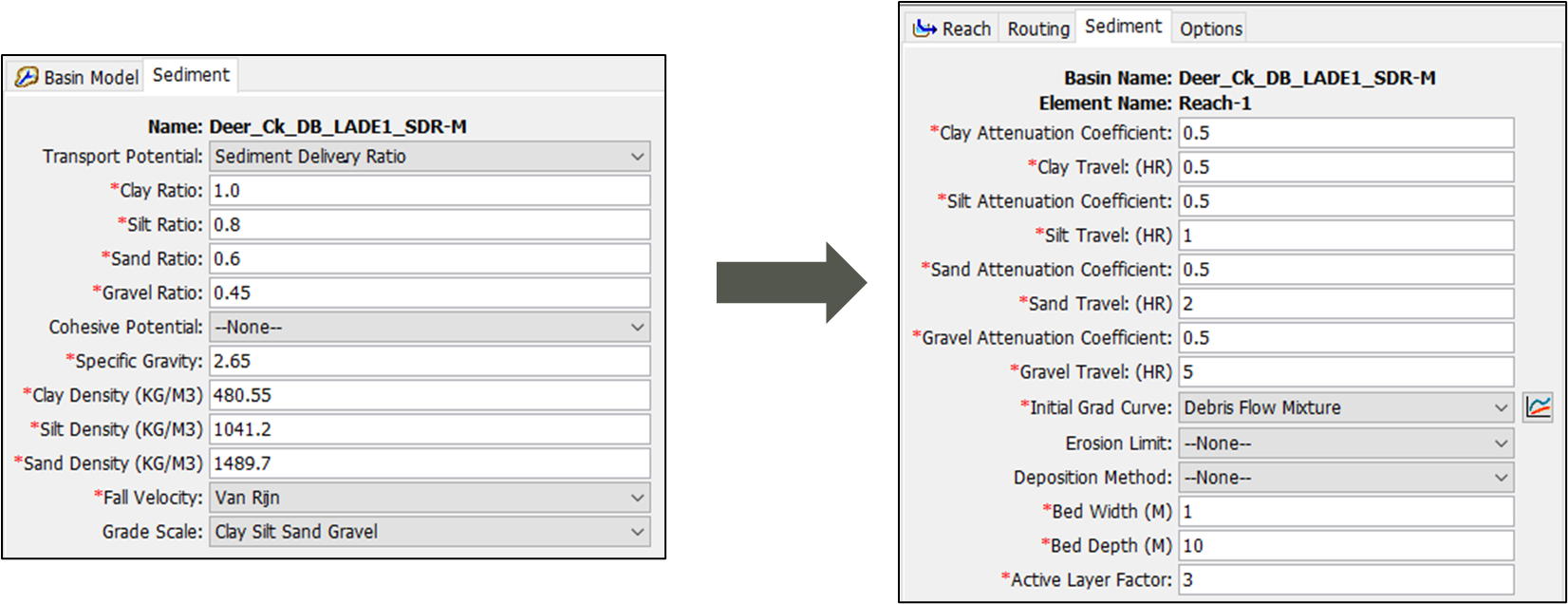
- On the Sediment tab, change the Transport Potential Method to Sediment Delivery Ratio and populate initial parameters values as shown below. Make sure the following options are selected.
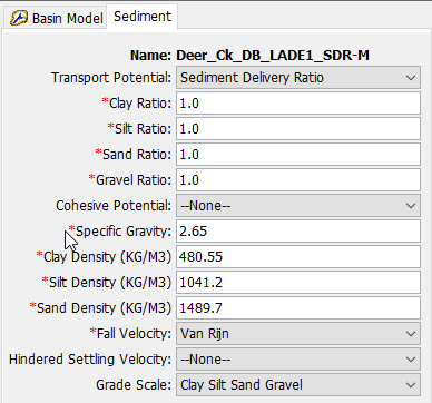
- Transport Potential: Sediment Delivery Ratio (designed for Debris Flow/Hyper-Concentration Flow)
- Clay Ratio: 1.0 (Initial value that will be calibrated)
- Silt Ratio: 1.0 (Initial value that will be calibrated)
- Sand Ratio: 1.0 (Initial value that will be calibrated)
- Gravel Ratio: 1.0 (Initial value that will be calibrated)
- Cohesive Potential: None
- Specific Gravity: 2.65 (Default Value)
- Clay Density (KG/M3): 480.55 (Default Value)
- Silt Density (KG/M3): 1041.2 (Default Value)
- Sand Density (KG/M3): 1489.7 (Default Value)
- Fall Velocity: Van Rijn
- Hindered Settling Velocity: None
- Grade Scale: Clay Silt Sand Gravel
- Calculate Relief Ratio using the characteristics of subbasin elements by selecting Parameters | Characteristics | Subbasin.
- Convert Relief Ratio from dimensionless unit to M/KM by multiplying 1000.
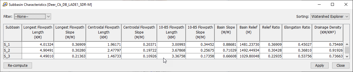
- Convert Relief Ratio from dimensionless unit to M/KM by multiplying 1000.
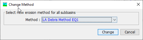
- Set the Erosion method to LA Debris Method EQ1 by selecting Parameters | Erosion | Change Method. As shown below, choose the LA Debris Method EQ1 and click the Change button. The erosion method will be set for all three subbasins.
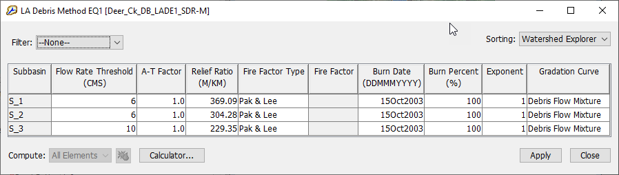
- Populate the initial subbasin parameters based on the given field data shown below. Open the global editor by selecting Parameters | Erosion | Los Angeles Debris Method EQ 1. Erosion parameters are described in the User's manual.
- A-T Factor: 1.0 (Set "1" as the default)
- Relief Ratio (M/KM): from the Subbasin Characteristics table
- Fire Factor Method: Pak & Lee Fire Factor
- Date (DDMMMYYYY): 15Oct2003 (from Fire record)
- Percent: 100 (from Fire Map)
- Flow Rate Threshold (M3/S): 6 (S_1), 6 (S_2), and 10 (S_3)
- Exponent: 1 (Default Value)
- Gradation Curve: Debris Flow Mixture (Generally, the gradation curve is generated based on field soil sample data at the debris basin. However, since field data was unavailable, this curve was created based on assumptions and only included silt, sand, and gravel.)
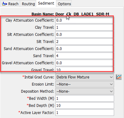
- On the Reach tab, change the Sediment Method to Muskingum.
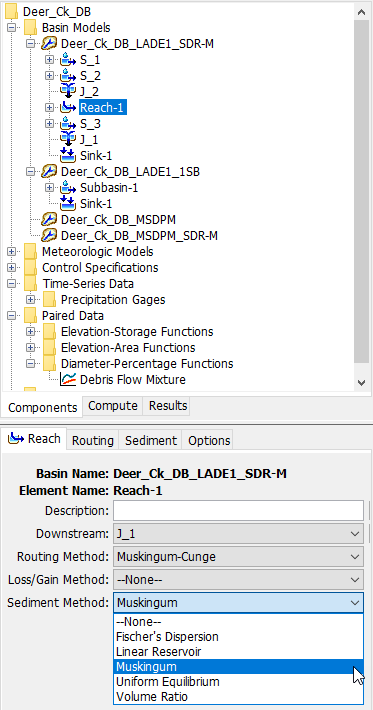
- Select the Sediment tab.
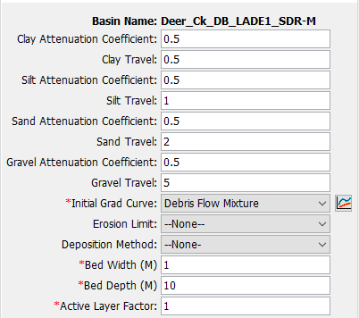
- Populate the initial reach sediment parameters based on the given data shown below. Sediment parameters are described in the User's manual.
- Attenuation Coefficient: 0.5 for all grain sizes (Initial value that will be calibrated. It ranges from 0.0 up to 0.5. A value of 0.0 results in maximum attenuation and 0.5 results in no attenuation)
- Travel (HR): 0.5 (Clay), 1 (Silt), 2 (Sand), and 5 (Gravel) (Initial value that will be calibrated)
- Initial Gradation Curve: Debris Flow Mixture
- Erosion Limit: None
- Deposition Limit: None
- Bed Width (M): 1 (Assumed value because there is no field survey data)
- Bed Depth (M): 10 (Assumed value because there is no field survey data)
- Active Layer Factor: 1
- Run LADE1_SDR-M by selecting Run: LAEQ1_SDR_M then click the raindrop icon
 .
.
- Compare the initial results with measured data.
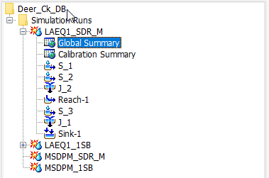
- Go to the Results tab and click on the Global Summary.
- The Global Summary has the results for the Sediment Volume of each subbasin, reach, and junctions with the Volume Units: 1000M3.
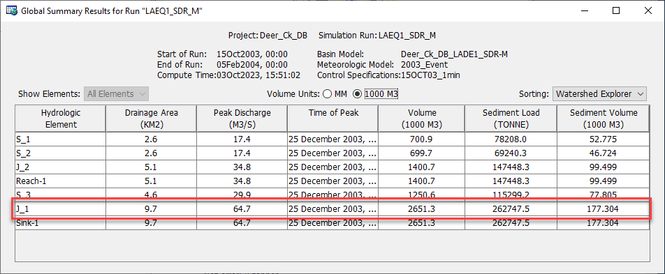
- Calibrate the model to match debris volume at Deer Creek Debris Basin (J-1) with the measured debris volume (120,112 m3) by changing the delivery ratios for Silt, Sand, and Gravel as shown below. (For training purposes, three delivery ratios for the Silt, Sand, and Gravel were selected for the model calibration.)
- Go to the Results tab and click on the Global Summary.
Question 1: What is the difference between your calculated debris volume and measured debris volume (120,112 m3)?
Difference: -0.6% with 0.6 for Silt, 0.4 for Sand, and 0.1 Gravel. (This will be one of possible answers but the answer will be different in different situations.)
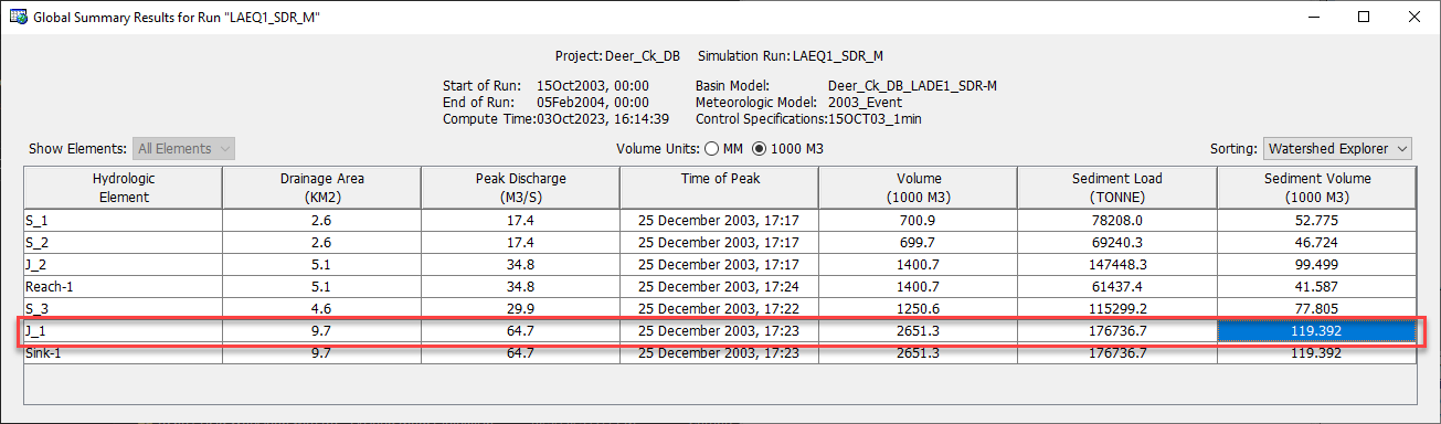
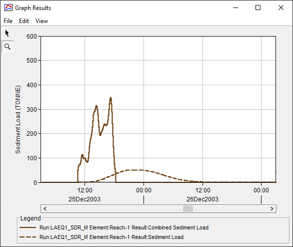
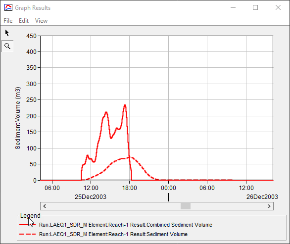
Question 2: How much debris volume deposited in the channel (Reach-1)?
Combined Sediment Loads from S_1 and S_2: 52,775 m3 (S_1)+ 46,724 m3 (S_2) = 99,499 m3
Sediment Load from Reach-1: 41,587 m3
Deposited Debris Volume in Reach-1: 57,912 m3
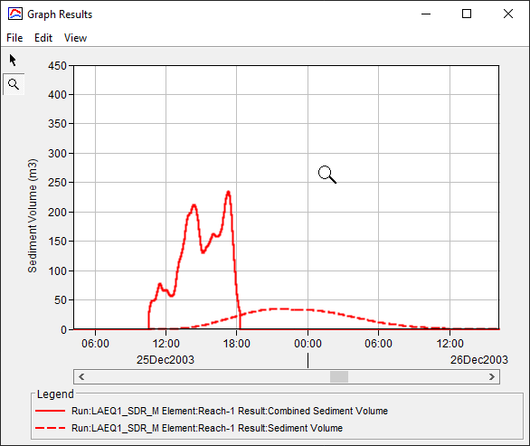
Question 3: Try to simulate a slow muddy flow situation (Non-Newtonian Flow) with the maximum attenuation (Attenuation Coefficient: 0.0) and doubled travel times. Do you think this Muskingum method can simulate muddy flow situations (Non-Newtonian Flow)?
The Muskingum Sediment Delivery Ratio method can be used to "simulate" Non-Newtonian Flow by increasing attenuation and travel time; however, hyper-concentrated flow can change between non-Newtonian and Newtonian flow as the flow travels downstream. This cannot be simulated using the Muskingum SDR method at this time.
Sediment Load (Before) Sediment Load (After)
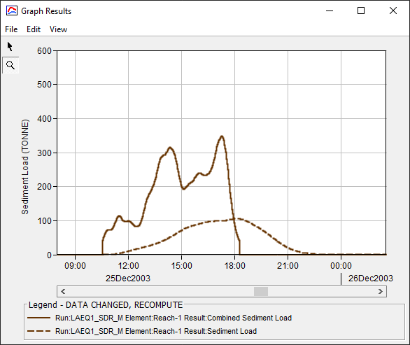
Sediment Volume (Before) Sediment Volume (After)
Question 4: What do you think is the biggest limitation to using the SDR transport potential method for reach elements in HEC-HMS?
Sediment Delivery Ratio values cannot be controlled for each reach element. We would need to move the transport potential methods, such as the SDR method, from the basin level to the element level (future development plan).
Question 5: Review the simple basin model that uses LA Debris EQ 1 Method with 1-subbasin (Deer_Ck_DBLADE1_1SB) and compare it with the Deer_Ck_DB_LADE1_SDR-M Basin Model (3-subbasin and 1-reach). What is the difference between the two models? How much debris volume deposited in the channel (Reach-1)?
| Deer_Ck_DBLADE1_1SB | Deer_Ck_DB_LADE1_SDR-M | |
|---|---|---|
| Pros |
|
|
| Cons |
|
|
Additional Tasks: If you are interested in other debris yield methods (MSDPM), please follow the above steps with the Deer_Ck_DB_MSDPM_SDR-M and Deer_Ck_DB_MSDPM basin models. With these additional tasks, you can see differences among four different methods and determine the best debris flow simulation result.