Download PDF
Download page Applying the Linear Deficit and Constant Loss Method.
Applying the Linear Deficit and Constant Loss Method
Last Modified: 2024-10-25 16:50:56.41This tutorial demonstrates the Linear Deficit and Constant loss method in HEC-HMS.
Software Version
HEC-HMS version 4.12 beta 1 was used to create this example. You can open the example project with HEC-HMS 4.12 beta 1 or a newer version.Overview
In this tutorial, you will apply the HEC-HMS linear deficit and constant loss method to a modeling application. The model will be calibrated using an optimization trial. You will run both event-based and continuous simulations.
Background
The linear deficit and constant loss method (LC method) is a modification of the initial constant loss method. It accounts for changes in infiltration capacity (or potential infiltration rate) as a function of cumulative infiltration and can be applied as an event-based or continuous model.
Event-Based Simulation
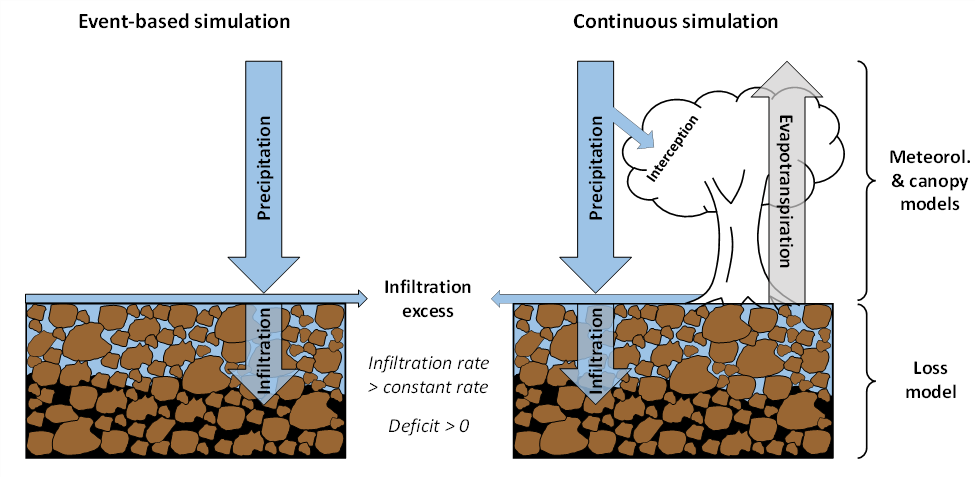
The LC method accounts for a single, hypothetical soil layer, hereafter referred to as the active soil layer. The soil layer has a maximum capacity to hold water. The figure below shows a conceptual representation of the linear deficit and constant loss method when the active soil layer is not completely saturated, i.e. the layer contains less water than the maximum storage capacity. The deficit, measured in millimeters or inches, is the amount of water required at any point in time to bring the active layer to saturation. During event-based simulation (left side of figure), water will infiltrate into the soil at a rate determined by the initial deficit, decay factor, and cumulative infiltration since the onset of the storm. If at any point in time the precipitation rate exceeds the potential infiltration rate, the difference (also called infiltration excess) will become runoff. If the precipitation rate at a given time is equal to or less than the potential infiltration rate, all rainfall will infiltrate into the soil.
Continuous Simulation
The LC method also allows for continuous simulation (see right side of the above figure) when used in combination with a canopy method that allows extraction of water from the soil due to evapotranspiration. Continuous simulation requires the specification of another loss parameter, the maximum deficit. This value can be interpreted as the porosity multiplied by the thickness of the active layer and is measured in millimeters or inches.
For continuous simulation, the modeler must select a canopy method (under subbasin elements) and specify an evapotranspiration (ET) method (under meteorologic models). ET removes water from the active soil layer between and, depending on user setting, optionally during storm events. The potential evapotranspiration rate is taken from the meteorologic model, where a variety of methods are available for representing that process. The ET rate is used as specified by the meteorologic model without any modification. There is no further evapotranspiration after the water in the soil layer is reduced to zero. Evapotranspiration will start again as soon as water is present in the soil layer. Unless a canopy and ET method are selected, no soil water extraction will occur. The canopy method also allows the modeler to simulate interception, the portion of precipitation intercepted by vegetation that never reaches the ground.
Percolation
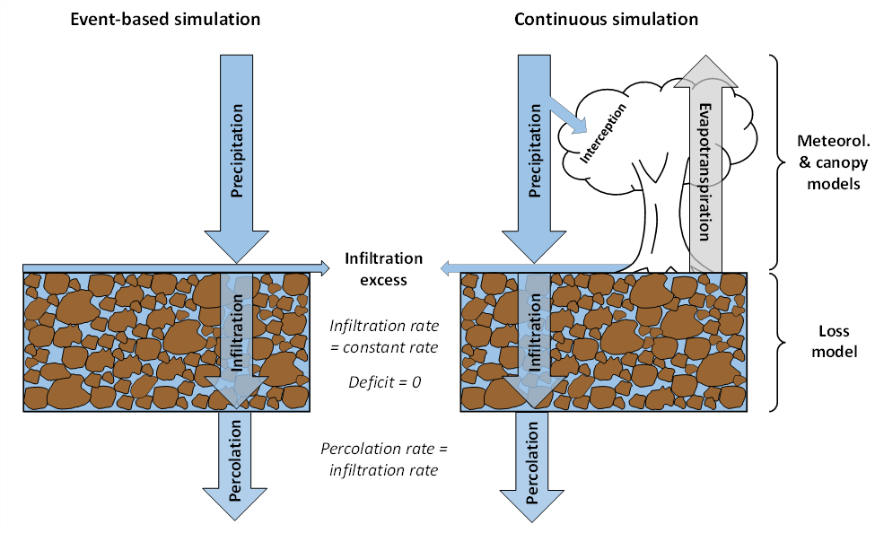
Once the active layer has saturated (the deficit is equal to zero), the potential infiltration rate becomes equal to the constant rate. Water will percolate out of the bottom of the active soil layer at a rate equal to the actual infiltration rate (see figure below). Percolation water is lost from the system. Percolation will continue as long as the soil layer is at maximum storage capacity (saturated), and precipitation continues. The linear deficit and constant method should therefore not be used for systems were (1) the water table is close to the surface, and the vadose zone could saturate completely during the analysis period; or (2) an impermeable layer is present at a depth sufficiently shallow that a perched aquifer could form during the analysis period. In both cases, there would be no percolation once the active layer is saturated, and all additional precipitation would become runoff.
Required Parameters
Parameters required to utilize this method within HEC-HMS include the initial deficit (mm or in), maximum deficit (mm or in), constant rate (mm/hr or in/hr), decay factor (1/hr) and directly connected impervious area (percent).
Study Area
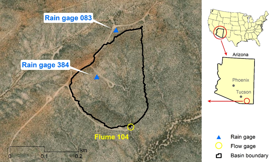
The study area for this tutorial is basin 104 within the Walnut Gulch experimental watershed near the city of Tombstone, Arizona (shown below). The basin has a size of 4.4 ha (0.044 km2) and is instrumented with two rain gages and a flume to measure runoff. Rain gage 083 is also equipped with a soil moisture probe at a depth of 5 cm. Data for the watershed can be obtained via the Southwest Watershed Research Center Data Access Project (https://www.tucson.ars.ag.gov/dap/). Soils in the basin are gravely sandy loams.
Estimate Initial Parameter Values
The parameter values presented in this section are intended as initial estimates only for the soil textures specified. Parameter guidance was developed for bare or sparsely vegetated soil plots in New Mexico under simulated rain. Evidence suggests that infiltration models can be parameterized successfully using plot-scale simulation under certain circumstances (Schoener et al., 2021). Nevertheless, initial estimates should be calibrated and validated using measured rainfall-runoff data whenever possible.
Initial Deficit
The initial deficit is the soil moisture deficit of the active soil layer at the onset of a storm event. The potential infiltration rate decreases linearly with cumulative infiltration until the initial deficit is satisfied. Once satisfied, the potential infiltration rate becomes constant (see constant rate below).
The table below provides estimates for the initial deficit parameter for different antecedent soil moisture conditions and texture classes sand, sandy loam, and loamy sand. The values are based on plot-scale rainfall simulator testing (Schoener et al., 2023) carried out at different test sites in New Mexico. The table contains median values, with reasonable ranges included in parenthesis. Rainfall simulator testing also revealed that physical soil crusts can substantially increase runoff, and crusted soils may be modeled equivalent to wet soils.
Proposed values for initial deficit, sand, loamy sand, and sandy loam texture classes.
Antecedent soil moisture | Initial deficit |
0.02 | 48 (36-72) |
0.06 | 36 (23-66) |
0.10 | 23 (10-54) |
0.14 | 10 (0-41) |
0.18 | 0 (0-28) |
0.22 * | 0 (0-16) |
* or presence of physical soil crust
Maximum Deficit
The maximum deficit specifies the maximum soil moisture deficit of the active soil layer. This value must be equal to or larger than the initial deficit. For event-based simulations, it will not impact model results. The maximum deficit can be interpreted as the porosity multiplied by the thickness of the active layer. Table 1 suggests a reasonable maximum deficit range for sands, sandy loams and loamy sands of 36-72 mm based on plot-scale rainfall simulator testing.
Decay Factor
The decay factor is the rate of infiltration potential decay with respect to cumulative infiltration. The default value is -3, but users can change decay factor values within the range of 0 to -8. Sensitivity analysis has shown that the LC loss method is substantially more sensitive to the initial deficit parameter compared to the decay factor, and that the latter may be held constant at -3 (paper under review).
Constant Rate
The constant rate determines the potential rate of infiltration that will occur after the initial deficit is satisfied. The same rate is applied regardless of the length of a simulation. The constant rate can be interpreted as the average effective hydraulic conductivity of the active soil layer. The following table specifies proposed values of the constant rate parameter for texture classes sand, sandy loam, and loamy sand.
Proposed values for constant rate parameter, sand, loamy sand, and sandy loam texture classes.
Texture class | Constant rate |
Sand | 31 (19-44) |
Loamy sand | 20 (14-26) |
Sandy loam | 15 (11-21) |
Directly Connected Impervious Area
The percentage of the subbasin comprised of directly connected impervious area can be specified. Directly connected impervious areas are surfaces where runoff is conveyed directly to a waterway or stormwater collection system. These surfaces differ from disconnected impervious areas where runoff encounters permeable areas which may infiltrate some (or all) of the runoff prior to reaching a waterway or stormwater collection system. No loss calculations are carried out on the specified percentage of the subbasin; all precipitation that falls on that portion of the subbasin becomes excess precipitation and subject to direct runoff.
Question 1: We will first model a time period spanning approximately 5.5 days (Jul 25 2010, 13:00 – Jul 30 2010, 00:00) using continuous simulation. From soil survey data, you know the soils in the study area are sandy loams not impacted by a physical soil crust. You also have soil moisture data for the period in question (see the SoilMoisture.xlsx spreadsheet at the beginning of the tutorial). Given the guidance provided above, what value would you use for the initial deficit parameter?
Based on the table above and an antecedent soil moisture state of 0.09 m3/m3, a value of 26 mm can be used as a first estimate for the initial deficit parameter (obtained by linear interpolation).
Question 2: What values would you use as a first guess for model parameters maximum deficit, decay factor, constant rate, and percent directly connected impervious area?
Maximum deficit: 48 mm (based on first table)
Decay factor: -3 (see discussion above)
Constant rate: 15 mm/hr (see second table, sandy loam)
Directly connected impervious area: 0% (it is apparent from the aerial image that no impervious surfaces are present in the study area)
Modify the Existing HEC-HMS Project
Now that you have estimated the initial parameters, begin modifying the existing HEC-HMS project.
- Open the LC_WalnutGulch project, then open the WalnutGulch_basin104 basin model.
- Select the basin_104 subbasin element.
- On the Subbasin tab, verify the loss method is set to Linear Deficit and Constant.
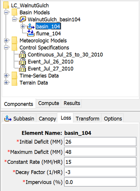
- Select the Loss tab to open the Linear Deficit and Constant Component Editor (shown below).
- Enter the initial deficit, maximum deficit, constant rate, decay factor, and percent directly connected impervious area.
- Review the Canopy and Transform tabs, where parameters have been pre-populated for you. The canopy method does not account for interception (both initial and maximum storage are set to zero) because the study area is sparsely vegetated.
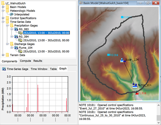
- Review Precipitation and Discharge data, which has also been pre-populated (shown below). Data from two precipitation gages and one discharge gage are available for the study area. Four distinct rain events with short duration and high precipitation intensities occurred during the study period, typical for the summer monsoon season in the Southwestern US. (Data source: Goodrich et al., 2008, Stone et al. 2008).
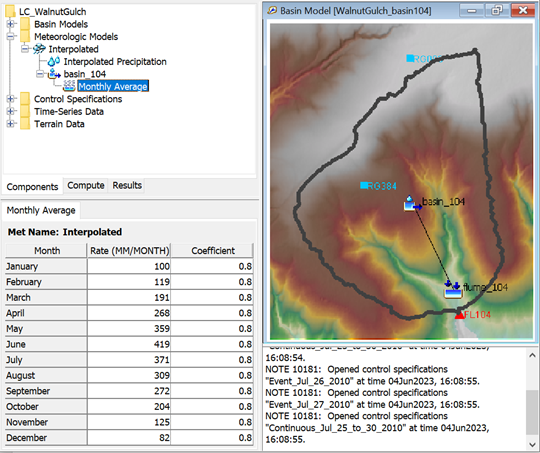
- Review the Meteorological model (shown below). It interpolates data from both precipitation gages using the inverse distance method, and accounts for evapotranspiration using the monthly average method (monthly pan evaporation values were obtained from the Western Regional Climate Center, https://wrcc.dri.edu/Climate/comp_table_show.php?stype=pan_evap_avg).
- Select the Continuous_Jul_25_to_30_2010 model run from the compute toolbar and press the Compute All Elements button to run the simulation.
- Click on the flume_104 sink element in the watershed explorer and view the results graph and summary table.
Question 3: What are the performance metrics (RMSE Std Dev, Percent Bias, and Nash-Sutcliffe efficiency for this model run? How would you assess model performance?
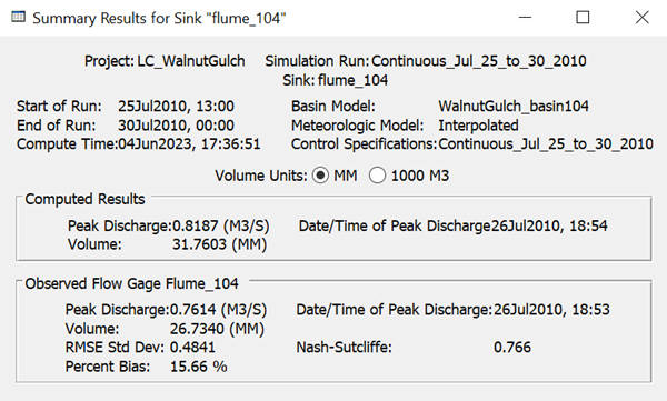
Based on initial parameter estimates, performance metrics are as follows (see Figure 6):
RMSE Std Dev = 0.48; bias = 16%, Nash-Sutcliffe efficiency (NSE) = 0.77. This is not a bad result for a first trial, particularly for a very flash ephemeral system. The model somewhat overestimates runoff volume and peak. NSE values greater than 0.5 are typically regarded as acceptable. Nevertheless, model performance can be improved by calibration.
Calibrate the Continuous Model
We will now use an optimization trial to calibrate the continuous model to improve model performance.
- In the watershed explorer, select the Compute tab and click on continuous_optimization under Optimization Trials folder (shown below). Many of the optimization trial parameters have been pre-populated for you.
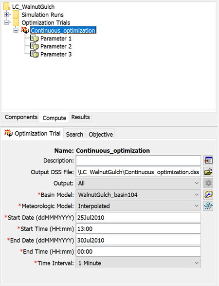
- Three parameters were included in the optimization trial: parameter: 1 = initial deficit; parameter 2 = maximum deficit; parameter 3 = constant rate. Click on each parameter in turn to view the component editor options. Notice the initial parameter values and the minimum and maximum values.
- Save and run the optimization trial.
Question 4: Even when measured data is available for model calibration, modelers often face challenges due to equifinality: different parameter combinations can produce similar outcomes, and it is difficult to ascertain which parameter set represents the best physical representation of the system. To reduce uncertainty due to equifinality, it is beneficial to constrain parameter ranges during calibration (see Beven & Freer, 2001; Mai, 2023). Based on what you know about the watershed, along with the guidance provided in section 2 above, what parameter ranges would you chose for initial deficit, maximum deficit and constant rate?
Initial deficit: range = 13-57 mm (see the first table, using linear interpolation for an antecedent soil moisture value of 0.09 m3/m3). Maximum deficit: range = 36-72 mm (see the first table, range of values for smallest antecedent soil moisture content of 0.02 m3/m3). Constant rate: range = 11-21 mm/hr (see the second table, range for sandy loam).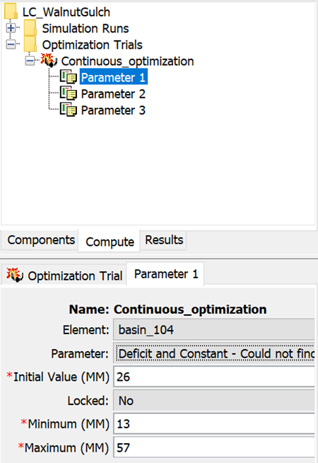
Question 5: In the watershed explorer, select the Results tab. Under Optimization Trials folder (see below), expand results for continuous_optimization. Here you have access to numerous summary statistics and detailed results for each model element. Review the Optimized Parameters summary table. What are the optimized parameters for initial deficit, maximum deficit, and constant rate? Next, look at the summary table for the element flume_104. Has model performance improved compared to your initial model run?
Optimized parameters: initial deficit = 32 mm, maximum deficit = 63 mm, constant rate = 20 mm/h.
Yes, all performance metrics have improved after calibration (see below).
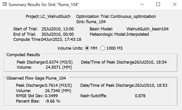
Due to the equifinality phenomenon discussed above, there may be other parameter combinations that produce model results with low error. It is therefore recommended to validate the model by applying parameters from calibrated model runs to other storm events and assess model performance. This exercise is left for the reader.
Run Event-Based Simulations
In this last exercise, we will use the same data applied to continuous simulation and run two event-based simulations for the two largest precipitation events: 18:30-20:00 on July 26, 2010, and 13:30-15:00 on July 27, 2010. Ideally, a separate basin model would be created for each historical event simulation to define the appropriate initial conditions. In this example, the same initial conditions will be used for both event-based simulations.
Question 6: Based on the soil moisture data for the period in question (see SoilMoisture.xlsx) and the first table, what initial deficit values would you use for the July 26 and 27 storms?
Antecedent soil moisture for both the July 26 and 27 storms is 0.09 m3/m3. Therefore, an initial deficit value of 26 mm can be used as a first estimate.
Verify that parameter values in the component editor for the linear deficit and constant loss method for subbasin basin_104 are set as shown below.
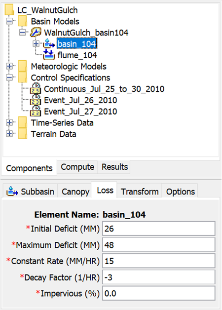
Run both event-based models (Event_Jul_26_2010 and Event_Jul_27_2010).
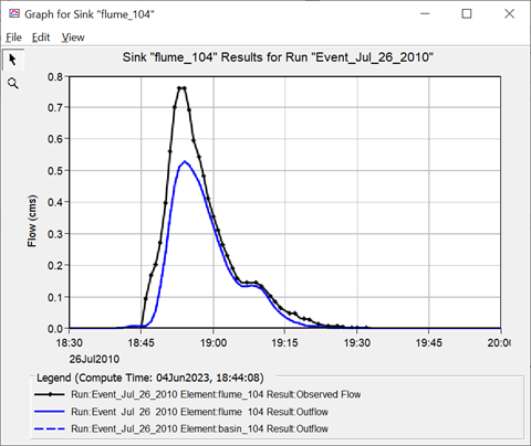
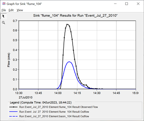
Question 7: Compare simulated and observed hydrographs for both event-based models. How well does the model perform using the initial parameter estimates? How could performance be improved?
The figure below shows simulated (blue) and measured (black) hydrographs for event-based simulations of the storms of July 26, 2010 (left) and July 27, 2010 (right). Both underestimate runoff, but hydrograph shape and timing is good. Model performance for event-based simulations can be improved using optimization trials.
References
Beven, K., & Freer, J. (2001). Equifinality, data assimilation, and uncertainty estimation in mechanistic modelling of complex environmental systems using the GLUE methodology. Journal of Hydrology, 249(1), 11–29. https://doi.org/10.1016/S0022‐1694(01)00421‐8
Goodrich, D. C., T. O. Keefer, C. L. Unkrich, M. H. Nichols, H. B. Osborn, J. J. Stone, and J. R. Smith (2008), Long-term precipitation database, Walnut Gulch Experimental Watershed, Arizona, United States, Water Resour. Res., 44, W05S04, doi:10.1029/2006WR005782.
Mai, J. (2023). Ten strategies towards successful calibration of environmental models. Journal of Hydrology, 620, 129414. https://doi.org/10.1016/j.jhydrol.2023.129414.
Schoener, G., Rassa, S., Fleming, M., Gatterman, D. and Montoya, J. (2023). Infiltration model parameters from rainfall simulation for sandy soils. Journal of Hydrologic Engineering. https://doi.org/10.1061/JHYEFF/HEENG-6025.
Stone, J. J., M. H. Nichols, D. C. Goodrich, and J. Buono (2008), Long-term runoff database, Walnut Gulch Experimental Watershed, Arizona, United States, Water Resour. Res., 44, W05S05, doi:10.1029/2006WR005733.
