Download PDF
Download page Using an HEC-RAS Model to Create Storage-Discharge Curves for Mod-Puls Reaches in HEC-HMS.
Using an HEC-RAS Model to Create Storage-Discharge Curves for Mod-Puls Reaches in HEC-HMS
This tutorial was developed using HEC-HMS 4.10 and HEC-RAS 6.2.
HEC-HMS version 4.10 and HEC-RAS version 6.2 was used to create this tutorial. You will need to use HEC-HMS version 4.10 and HEC-RAS version 6.2, or newer, to open the project files.
Download the initial project files here:

Introduction
This workshop will help you learn how to use output from HEC-RAS to set up routing reach properties in HEC-HMS. You will use the Modified Puls method to route a flood wave through a river reach and will check the amount of attenuation and lag time calculated for each reach. Storage-Outflow functions will be determined in HEC-RAS and imported into HEC-HMS for each routing reach. Results will be compared with an existing unsteady flow HEC-RAS model and HEC-HMS model parameters will be adjusted as necessary.
Background
The stream for this example is Bald Eagle Creek, which is a tributary of the West Branch Susquehanna River in central Pennsylvania. Bald Eagle Creek flows for 26 miles from the upstream end of Foster Joseph Sayers dam to the confluence with the West Branch of the Susquehanna River. For the purposes of this workshop, the dam was removed from the models, and the 26 miles of river will be modeled as separate routing reaches for comparison purposes.
Problem Description
An HEC-HMS project (BaldEagleCrClass) and a HEC-RAS project (BaldEagleClass) were included in the zip file at the beginning of this workshop. The objective of this workshop is to route a flood through Bald Eagle Creek using HEC-HMS. The event of interest has a duration of 48 hours and a peak flow of 60,000 cfs, occurring at hour 24. This hydrograph is already input to DSS and referenced in the HEC-HMS project using a Source element. Bald Eagle Creek will be divided into 5 reaches for the Modified Pulse Routing. For each reach you will have to estimate an appropriate number of sub-reaches. HEC-RAS can be used to develop a series of flow profiles for different discharges. From these profiles, the volume, or storage between two points on a stream can be determined for any amount of discharge. This relationship can then be input to the routing reach properties of the Modified Puls method in HEC-HMS. You will determine the attenuation and lag times for each reach and for the entire stream. The HEC-HMS model will be calibrated to an existing HEC-RAS unsteady flow model by adjusting the number of sub-reaches in each reach. We are assuming that the unsteady flow model results are a good representation of how a flood wave will move through this stream system.
Tasks
The following are the required tasks for this workshop:
- Run a steady flow analysis of Bald Eagle Creek in HEC-RAS.
- Export HEC-RAS data to a DSS file.
- Import Storage-Discharge Functions with the HMS Paired Data Manager.
- Finish the Data for each of the Routing Reaches
- Run a simulation in HMS.
- View the Output and Analyze the Results.
Run a steady flow analysis of Bald Eagle Creek in HEC-RAS
The data is already entered in the RAS project file called BaldEagleClass.prj. This task will require students to review the entered data prior to developing storage-discharge functions.
- Open up HEC-RAS.
- Open the project C:\...\BaldEagleCrClass_Initial\HEC-RAS\BaldEagleClass.prj (File | Open Project) from the workshop directory.
- View the geometry (Edit |Geometric Data). This will provide a plan view of the Bald Eagle Creek. You can also view a 3-D perspective plot (View | X-Y-Z Perspective Plots).
- Check the Steady Flow Setup. Make sure 11 profiles are included from the 0.5 to the 500 year event. (Edit | Steady Flow Data)
- Run the computation. (Run | Steady Flow Analysis). Make sure subcritical is selected and then press Compute. When the computations are complete, close the Hydraulic Computations Window.
- Review the results. Plot the water surface profiles. (View | Water Surface Profiles). Select only the 500-yr event (Options | Profiles) by clearing all selected profiles and then double-clicking 500-yr profile under the available profiles window.

Export HEC-RAS data to a DSS file
Now that the computations are complete, the storage-discharge functions will be exported to a DSS file.
- Open up the Export to DSS window and enter in the reach information to be exported to DSS. From the main RAS window select File | Export to HEC-DSS. The DSS path and filename should be similar to "C:\Temp\BaldEagleCrClass_Initial\HEC-HMS\data\BaldEagleClass_Export.dss". Since we will be using this exported data within our HEC-HMS project, it's good practice to save the data within the HEC-HMS project's directory (save the file to the project's data folder). Click on the Storage-Outflow tab and enter the data as shown in the figure below.

- Export the data to DSS. Press the Export Volume Outflow Data. If the 5 reaches are shown in the window, press Close. Then Press OK in the Exporting to DSS window to get out of the editor.
Import Storage-Discharge Functions with the HMS Paired Data Manager
Getting storage outflow data into HMS for use in a routing reach is a two step process. First a place holder, name, and description is established using the Paired Data Manager. Then a data source is established for each paired data place holder (entered in a table or linked to a DSS record). The following are the steps to bring in the data through the paired data manager and link each curve to a DSS record:
- Start the HMS software and load the project C:\...\BaldEagleCrClass_Initial\HEC-HMS\BaldEagleCrClass.hms (File | Open).
- View the Basin model labeled “Uncalibrated Routing”, to see the hydrograph source (Source -1), routing reaches (Reach-1 through Reach-5), and the downstream outlet (D.S. Outlet).
- Go to the Components menu and selected the Paired Data Manager. The Paired Data Manager will appear as shown in the figure below, except your window will be blank.

- Select Storage-Discharge Functions from the Data Type drop down box, then press the New button to enter a name and description for the first storage discharge curve. Use a name like “Reach 1” for the curve. Repeat this process for each of the five reaches. Once names and descriptions have been entered for each of the five storage discharge curves, the Paired Data Manager can be closed.
- The next step is to link each of the Paired Data storage discharge functions to the corresponding curve computed by HEC-RAS and stored in the DSS output file that we copied to the project's data folder. Go to the HEC-HMS watershed explorer tree and open the Paired Data folder, and then the Storage-Discharge Functions folder. Select the label for one of the Storage-Discharge Functions. The explorer and corresponding paired data editor should look as shown in the figure below.

- For each Storage-Discharge Function the user must select the Data Source – Data Storage System (HEC-DSS); the DSS filename - "BaldEagleClass.dss"; and then select the appropriate DSS Pathname stored in the DSS file. The DSS Pathname chooser is shown in the figure below.

- Select the HEC-RAS computed Storage-Discharge function that corresponds to the HEC-HMS Storage-Discharge Function you are currently working on. Remember that HEC-RAS labels the B-Part of the DSS pathname as the river stationing of the downstream cross section of the storage-outflow reach. For example, the pathname for the storage outflow curve that corresponds to the HEC-HMS routing reach labeled “Reach 1” is as follows:
/BALD EAGLE LOC HAV/103122.3/STORAGE-FLOW///STEADYFLOWRUN/ - Repeat the process of linking a DSS Pathname to an HMS Paired Data Function for each of the remaining routing reaches.
Finish the Data for each of the Routing Reaches
The next step is to enter all of the required data for the Modified-Puls method for each of the routing reaches. The following is a listing of the steps to do this:
- First select the upstream routing reach (Reach-1) from the basin model labeled “Uncalibrated Routing” using the watershed explorer (Basin Models | Uncalibrated Routing | Reach-1).
- Once the reach is selected, the component editor will show up in the lower left panel. The “Reach” tab should be selected by default. Make sure the Routing Method is set to Modified Puls.
- Select the Routing Tab, then for the field labeled “Stor-Dis Function”, select the appropriate storage discharge function for that reach. An example is shown in the figure below.

- For the field labeled “Initial Type” make sure it is set to Discharge = Inflow.
The final step is to select the number of subreaches to break the routing reach into for computational purposes. Select the number of subreaches for each reach as follows:
Number of Subreaches = K/ΔT
K = Travel time across the reach (determined from the HEC-RAS unsteady flow model)
ΔT = Time step (1hour for this simulation)Reach K (hrs) Number of Subreaches 1 1.95 2
2 1.77 2
3 1.60 2
4 2.82 3
5 6.57 7
Perform these steps to fill out the data for each routing reach.
Run a simulation in HMS
All remaining necessary data to run a simulation has already been entered into the HEC-HMS project.
- Make sure “Inflow” hydrograph is selected for the source. You can check this setting from the watershed explorer (Time-Series Data | Discharge Gages | Inflow). Its path name is /BALD EAGLE LOC HAV1/138154.4/FLOW//1HOUR/UNSTEADYFLOW/.
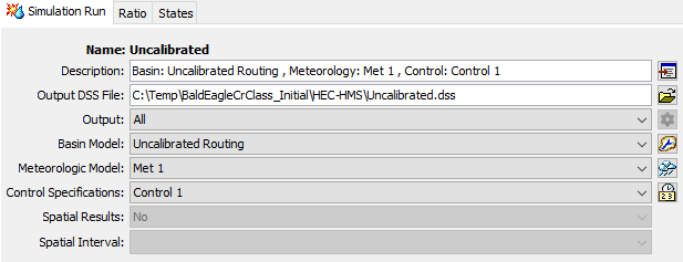
- A simulation run should already be created and called “Uncalibrated”. This simulation uses the “Uncalibrated Routing” Basin Model, “Met 1” Meteorologic Model, and “Control 1” Control Specifications.
- Run the simulation.
View the Output and Analyze the Results
A graph of the inflow and outflow hydrographs for reach 5 is shown in the figure below.

Additionally, the HMS Global Summary Results table is shown in the figure below.

What is the attenuation in Reach 1?
516 cfs
Reach 2?
339 cfs
Reach 3?
152 cfs
Reach 4?
324 cfs
Reach 5?
1299 cfs
What is the lag time through Reach 1?
2 hours
Reach 2?
2 hours
Reach 3?
1 hour
Reach 4?
2 hours
Reach 5?
6 hours
Why does Reach 5 show more attenuation than the other reaches?
Reach 5 is has a flatter slope than the other reaches, and is experiencing a significant backwater effect from its confluence with the West Branch of the Susquehanna River. This decreases the slope of the water surface in this location and therefore increases the available storage for a given discharge. This can be viewed in the profile chart in HEC-RAS. According to the continuity equation, for a given inflow, the outflow must decrease if the rate change of storage increases. O = I-ΔS/Δt

Compare the results with an unsteady flow HEC-RAS model. The method of selecting the number of subreaches is not always full proof. Plot the hydrographs for both the unsteady HEC-RAS model and the HEC-HMS simulation and look for reaches where the number of subreaches may need to be adjusted. Use HEC-DSSVue for the following steps.
- Open DSS file "BaldEagleCrClass.dss" in the HEC-HMS project directory. Select the path /REACH-1/FLOW/01FEB1999/1HOUR/RUN:UNCALIBRATED/.
- Open DSS file "BaldEagleClass.dss" in the HEC-HMS project's data directory. Select the path /BALD EAGLE LOC HAV/103122.3/FLOW/01FEB1999/1HOUR/UNSTEADYFLOW/.
- Plot the selected paths. Are there any discrepancies between the two hydrographs? If so, how would you adjust?
Repeat for reaches 2 through 5. The HEC-RAS hydrographs will be stored with the following B pathname part labels:
HMS Reach HEC-RAS Location Reach-1
103122.3 Reach-2 75917.82 Reach-3 58708.54 Reach-4 36339.56 Reach-5 659.942  Hydrographs for Reach 5.")
Notice that the unsteady flow model has a lower peak hydrograph than the HEC-HMS simulation for reach 5. Decreasing the number of subreaches for this reach will increase attenuation and bring the peak down to the desired level.
Adjust the number of subreaches where necessary and rerun the HEC-HMS model.
- Copy Basin 1 and name the new copy “Calibrated”.
- Adjust thesub reaches where necessary.
- Create a new simulation run (Compute | Create Compute | Simulation Run) named “Calibrated” that uses the new "Calibrated" basin model and the existing "Met 1" meteorologic model and "Control 1" control specification.
- Run the simulation.
Continue to adjust the subreaches until the HEC-HMS model is calibrated to the HEC-RAS unsteady flow model.

The HEC-HMS simulation of Reach 5 with 1 subreach produces a slightly lower peak flow than the unsteady flow simulation. Using 2 subreaches gives a hydrograph with a larger deviation from the unsteady flow hydrograph, and a higher peak. In this case, a judgment call is necessary that may involve investigating the stage/discharge relationship, the land-use characteristics, and other factors.
What was the number of sub reaches used in each reach for the new calibrated model?
| Reach | # Sub Reaches | Attenuation (cfs) |
|---|---|---|
| 1 | 2 | 516 |
| 2 | 2 | 339 |
| 3 | 2 | 152 |
| 4 | 2 | 484 |
| 5 | 1 or 2 | 7797 or 4657 |
For the reaches where the number of subreaches was adjusted, why did the methods used to estimate the number of subreaches not produce the best results?
The number of sub reaches was decreased to 2 in reach 4, and 1 or 2 in reach 5. The reason the estimation method method did not work for reaches 4 and 5 is because these reaches have shallow water surface slopes due to the mild bed slopes and downstream backwater effect. An incoming flood wave has more room to spread out and attenuate because these reach segments more resemble a reservoir than a free-flowing stream. Knowing whether a reach acts more like a free flowing stream or a reservoir takes some practice. This can be investigated by examining the cross sections for this reach in HEC-RAS. This indicates the importance of calibrating the HEC-HMS model to field data.