Applying the Interpolation Method to Create Gridded Temperature Datasets in HEC-HMS

HEC-HMS version 4.10 beta 5 was used for this example. 

Introduction

Utilizing gridded data in an HEC-HMS model better captures the meteorology temporally and spatially across a watershed when compared to gage measurements at a single point. However, hourly or sub-hourly gridded meteorology products, such as Multi-Radar Multi-Sensor (MRMS) Quantitative Precipitation Estimate (QPE), Snow Data Assimilation System (SNODAS), or Next Generation Radar (NEXRAD), are not always available, particularly for historic events of interest to the modeler. In these cases, a gridded dataset can be created by interpolating point observations recorded at weather stations.

In HMS version 4.10 and above, interpolated grids can be developed for shortwave radiation, precipitation, temperature, windspeed, dew point temperature, and evapotranspiration. This tutorial demonstrates how gaged temperature measurements can be interpolated to create a gridded temperature dataset and how it can be applied to snowmelt modeling using the Truckee River HEC-HMS model. The Truckee River basin, home to Lake Tahoe, is located in the Sierra Nevada mountains and straddles the border between California and Nevada. The figure below shows the location of all the temperature gages in the model relative to the Truckee River watershed. The lowest elevation in the watershed is 4,450 feet, and the highest elevation is 10,300 feet.

Download initial project files here - Truckee_River_Initial.zip

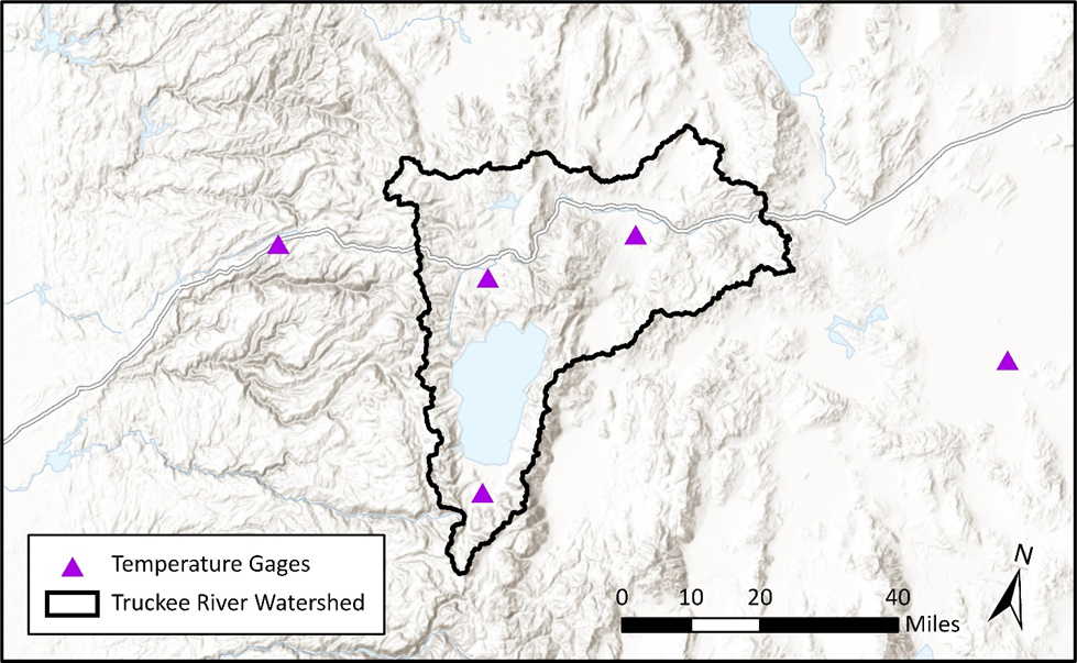
Inspect Temperature Data

1. Navigate to the data subfolder in the Truckee River model directory and open the Jan_1997_gage_temperature.dss file in HEC-DSSVue. Inspect the temperature time-series in the dss file. The E-part of the timeseries entry shows that all the gage data has an hourly timestep. The C-part of each timeseries is named TEMP-AIR, as shown below.
   
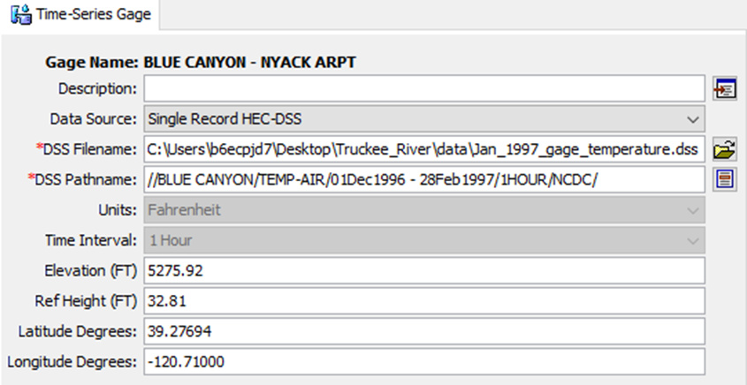
2. Open the Truckee_River HEC-HMS project and expand the Time-Series Data folder in the Watershed Explorer. Expand the Temperature Gages folder to see five temperature gages contained in the dss file. Select BLUE CANYON - NYACK ARPT temperature gage and look at its Component Editor. The following information must be set in order for the Interpolation Method to work.

   1. The latitude and longitude of each gage is entered either in Decimal Degrees or Degree-Minutes-Seconds. If the latitude and longitude are not specified, the gage cannot be used for interpolation.
      

      

      Within the General tab in the Program Settings editor, you can change the latitude and longitude to be displayed as either Deg Min Sec or Decimal Degrees

   2. The ground elevation of the temperature gage is enter in Elevation (FT). The height above the ground surface where measurements are taken is entered in the Ref Height (FT). 
      

Create an Interpolated Temperature Grid

Unlike other gridded data tools in HEC-HMS (like the Normalizer and Importer tools), the setup and specifications for gage interpolation are entirely contained within the method's Component Editor. The interpolation is conducted when a simulation using the Interpolation Method is computed. The interpolated grid files are written to the meteorological model’s dss file.

Configure the Meteorological Model

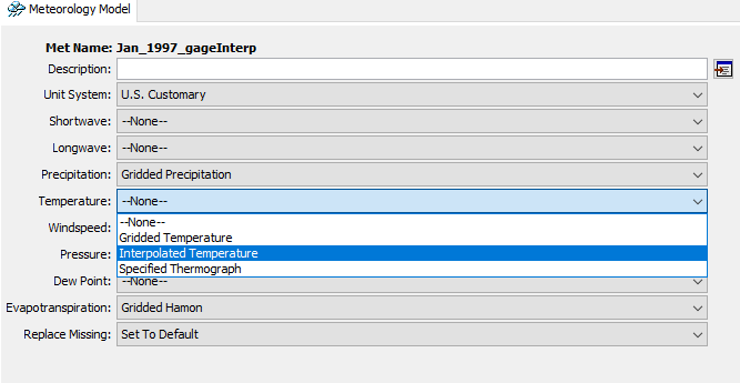
1. Select Jan_1997_gageInterp meteorologic model and inspect the Component Editor as shown below. Change Temperature to Interpolated Temperature.
   
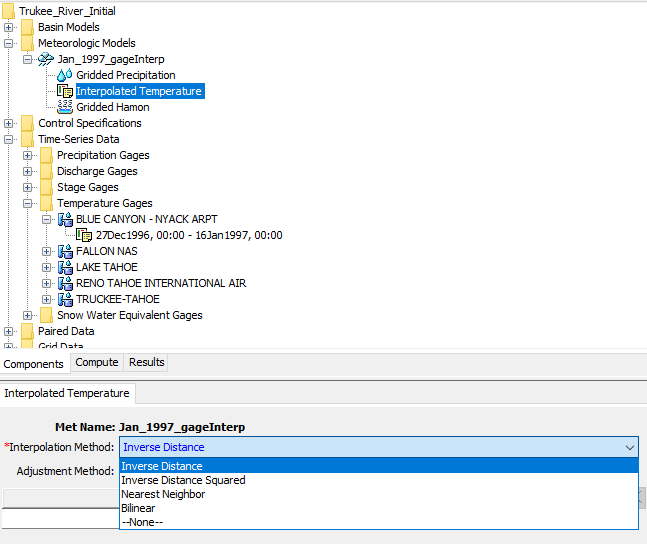
2. Select Interpolated Temperature in the Watershed Explorer and set the Interpolation Method to Inverse Distance. The Inverse Distance interpolation method assumes the weight, or influence, of a given measurement is equal to the inverse of its distance from the interpolated cell. Other interpolation methods, Inverse Distance Squared, Nearest Neighbor, and Bilinear, are also available and may be more applicable when interpolating grids for other climatological variables.
   
3. Set the Adjustment Method to Lapse and the Lapse Rate (DEG F/1000 FT) to -3.5, which is approximately the rate at which temperature changes with every 1,000 feet of elevation gain in this area. The lapse rate will adjust interpolated temperature throughout the basin model based on the terrain data.
   
4. In the table under Gage, select each temperature gage in the model, and assign it a radius of influence of 31 miles (50 kilometers). You should have a total of five gages listed in the table as shown below.
   
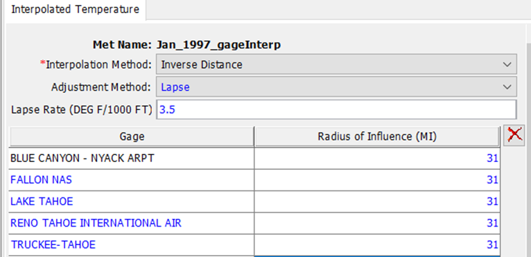
   The radius of influence, shown for each gage below, is the maximum interpolation distance. Beyond its radius of influence, the gage will not affect the cell values of the interpolated grid.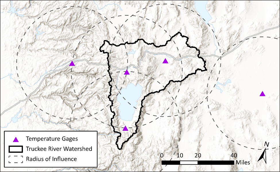 
   

If a gage does not have any data for a given timestep, that gage will be excluded from the interpolation for that timestep. A value of zero does not get skipped!

Compute the Interpolated Temperature Grids

To compute the interpolated grids, a simulation must be computed that uses the meteorological model.

1. At the bottom of the Watershed Explorer, navigate to the Compute tab. Expand the Simulation Runs folder and compute the Jan_1997_gageInterp simulation run by right-clicking on Jan_1997_gageInterp and clicking Compute.
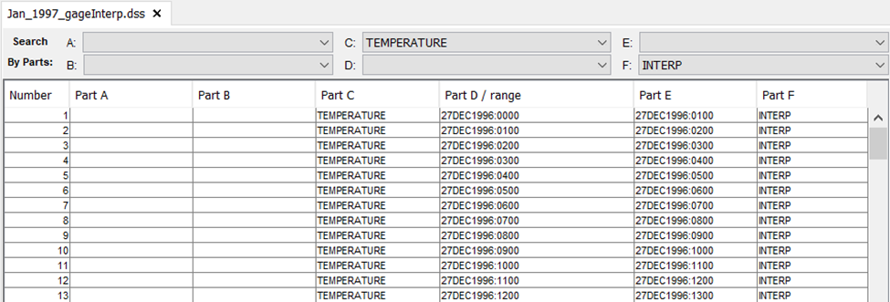
2. Once the compute is complete, navigate to the Jan_1997_gageInterp.dss file in the HEC-HMS project directory.
   
3. Open the Jan_1997_gageInterp.dss with HEC-DSSVue and filter to only include data with the C-part TEMPERATURE. All of the filtered files shown below are the interpolated temperature grid records.
   

View Simulation Results

The interpolated air temperature can be viewed in the HEC-HMS basin model map window. Spatial results must be turned on within the simulation run's Component Editor and the basin model must be georeferenced. I

1. Navigate to the Spatial Results Tool bar and select Air Temperature. Select OK on the Process Animation Tiles Window.
   

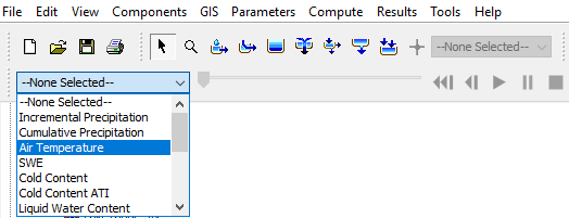
2. Once the process completes, the Map Window will be updated with temperature grid values along with a Air-Temperature legend (you must turn the legend on). Move the slider or press the play button located next to the Spatial Results toolbar to see air temperatures change across the basin.
   

   

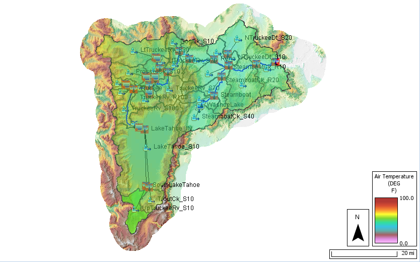
   Select the Spatial Results Toolbar Properties Symbology tab to change the temperature value range

3. You can right click within the spatial results grid and choose the Plot Spatial Results option to see a time-series plot for the selected grid cell.  
4. To view the subbasin-averaged temperature time-series, navigate to the Results tab at the bottom of the Watershed Explorer. Expand the Simulation Runs folder and expand the Jan_1997_gageInterp simulation. 
5. Expand any subbasin element and click on Air Temperature. The subbasin-averaged air temperature time-series will appear below.  
   
   
   

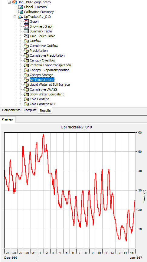
The gridded temperature values are based off of five point gages and a lapse rate but does not account for terrain slope direction, winds, and cloud cover. One method of validating interpolated temperature values is to compare values with other gridded temperature products, such as the daily temperature PRISM grids produced from Oregon State as shown below for subbasin UPTRUCKEEV_S10 (the Grid to Point tool was used to process the PRISM grids and compute subbasin average temperature time-series).  

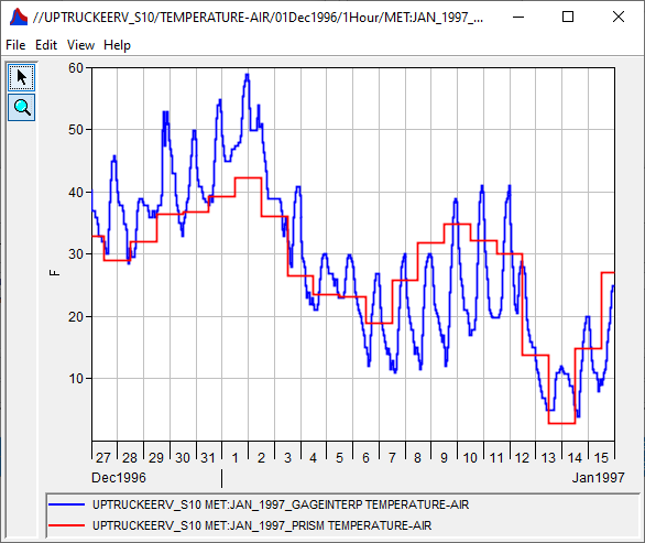
The PRISM daily subbasin-averaged temperatures are shown in red while the simulated HEC-HMS subbasin-averaged temperature results are shown in blue. The interpolated temperatures are generally higher than PRISM temperatures for the first part of the event in late December to early January and lower than PRISM temperatures for the second part of the event. To further improve the simulation results, you can try using other interpolation methods, adjust the radius of influence for certain gages, or gather additional point temperature data.  

Download final project files here - Truckee_River_Final.zip