Download PDF
Download page Using a Single Gage within the Interpolated Grid Option.
Using a Single Gage within the Interpolated Grid Option
HEC-HMS version 4.10 beta 4 was used to develop this tutorial.
Download the initial HEC-HMS project files here - Success_Dam_initial.zip
Introduction
A new interpolation option was added to the meteorologic model in HEC-HMS version 4.10. You now have the option to select point gage data and HEC-HMS will interpolate the point data to cover elements in the basin model. There is an option to use terrain and a lapse rate when interpolating temperature gage data, and the program contains an option for including a bias grid when interpolating precipitation gages. In order to use the new interpolation options, the basin model must be georeferenced. The discretization method is used by the interpolation process. For structured and unstructured discretization methods, the program will create an interpolated surface using the centroid of each cell. When no discretization method (subbasin average) is selected, the program will interpolate the gage values to the centroid of each subbasin.
The goal of this example application is to demonstrate how to apply the new interpolation option and show how helpful the bias option can be when interpolating precipitation data in mountainous terrain. Some simplifications in the modeling process were made in the example. For example, only one precipitation and temperature gage were used for interpolation. It is recommended that you use as many quality measurements as possible when developing boundary conditions for a hydrologic model.
Background
The Tule River watershed upstream of Success Dam is used for this example. The watershed is approximately 390 square miles and is located in the central Sierra Mountains in California. Elevation ranges from 650 feet at the dam to over 8,000 feet along the watershed boundary. The figure below show the watershed delineated into six subbasins. A major flood, rain on snow condition, occurred in January 1997 and is simulated in the model. You will notice in the basin model that there are three locations, junctions, with observed flow. These are the TuleR_MF_Gage, TuleR-R20, and TuleR_SF_Gage junction elements.
The figure below also shows locations for a precipitation gage (springville rs) and a temperature gage (Wet Meadows). Both gages have already been added to the project. The latitude and longitude were entered for the gages, and an elevation of 8,900 feet was defined for the temperature gage. 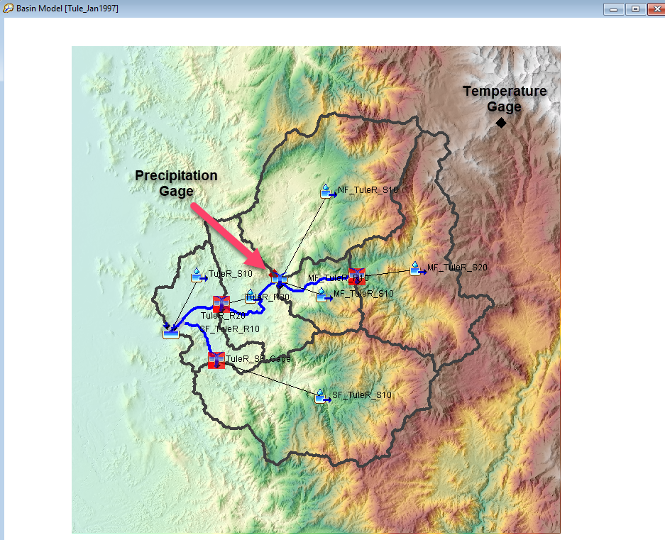
The gridded temperature index snowmelt method has already been configured within the basin model. The initial Snow Water Equivalent (SWE) was gathered for December 26, 1996, and then default conditions were used for the other snow state variables.
A raster dataset of the total precipitation for the January 1997 flood event, including the period leading up to the flood, was imported into the project (it is the 97 storm total Precipitation-Normal grid). The figure below shows the total storm precipitation was the highest, around 10 inches, at the highest elevations and was the lowest, around 2.5 inches at the watershed outlet. The precipitation gage is located in the 4 - 6 inch precipitation band (the gage recorded 3.3 inches of precipitation). The gridded data import tool was used to import the total storm precipitation (saved as a *.tif file) into a gridded DSS record. Then the total storm precipitation grid was added to the Success_Dam project as a Precipitation-Normal Grid. 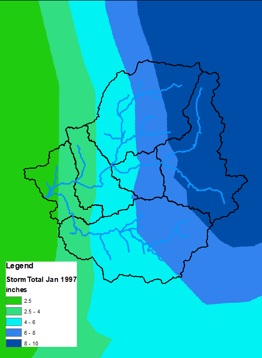
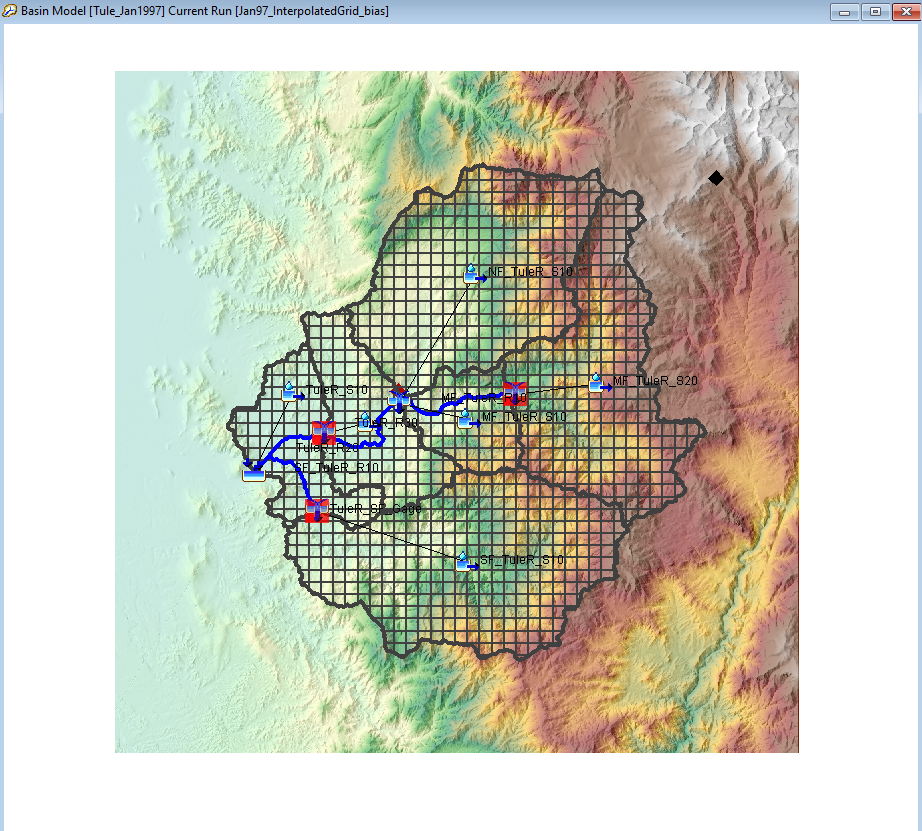
If you turn on the Discretization map layer your basin model map should look similar to the figure below. A 1,000 meter SHG was selected for each of the six subbasin elements.
Extents of background data used for interpolation
It is required that all background datasets used in the interpolation process be extended beyond the watershed boundary. For example, the terrain dataset should extend beyond the watershed boundary so that the centroid of each SHG cell is located on top of the terrain dataset. Also, the bias grid must cover all precipitation gages as well.
Task 1 Configure the Gridded_Jan1997_bias and Gridded_Jan1997 Meteorologic Models
Two simulations have already been configured for you. The only difference in the two simulations is that the Jan97_InterpolatedGrid_bias simulation uses the Gridded_Jan1997_bias meteorologic model and the Jan97_InterpolatedGrid simulation uses the Gridded_Jan1997 meteorologic model. Both simulation have the option turned on to save spatial results.
- Open the Component Editor for the Gridded_Jan1997_bias meteorologic model.
- Change the Precipitation method to Interpolated Precipitation.
- Change the Temperature method to Interpolated Temperature.
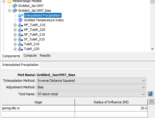
- Expand the Gridded_Jan1997_bias node in the Watershed Explorer and click on Interpolated Precipitation to open the Component Editor.
- As shown in the figure below, set the Interpolation Method to Inverse Distance Squared (the method does not matter for this example since only one gage is used for interpolation), choose the Bias Adjustment Method, and choose the 97 storm total bias grid. In the bottom table, select the springville rs precipitation gage and enter a Radius of Influence of 20 miles. A 20 mile radius is large enough for the springville rs gage to cover all SHG cells in the watershed.
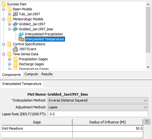
- As shown in the figure below, set the Interpolation Method to Inverse Distance Squared (the method does not matter for this example since only one gage is used for interpolation), choose the Lapse Adjustment Method, and enter a lapse rate of -3 degrees Fahrenheit per 1,000 feet in elevation. In the bottom table, select the Wet Meadows temperature gage and enter a Radius of Influence of 50 miles. A 50 mile radius is large enough for the Wet Meadows gage to cover all SHG cells in the watershed.
- Follow the steps above and configure the Gridded_Jan1997 meteorologic model. Do not select a Bias grid (no Adjustment Method) in the Interpolated Precipitation component editor. Make sure you use the same laps adjustment in the Interpolated Temperature Component Editor.
Task 2 Run Model Simulations and Compare Results
- Run both the Jan97_InterpolatedGrid and Jan97_InterpolatedGrid_bias simulations.
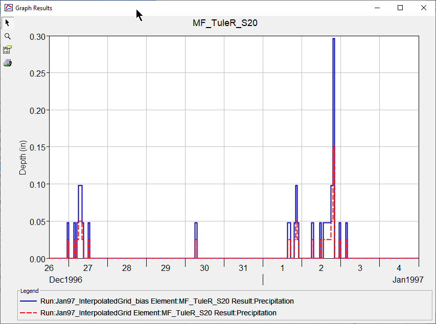
- Compare precipitation hyetographs at the MF_TuleR_S20 subbasin. As shown in the figure below, the MF_TuleR_S20 subbasin has more precipitation in the Jan97_InterpolatedGrid_bias simulation than in the Jan97_InterpolatedGrid simulation. Using the bias grid (the storm total grid) resulted in the basin average increasing to a total of 6.56 inches vs. 3.3 inches when no bias grid was used.
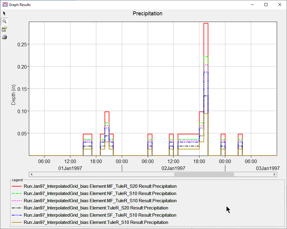
- The following figure shows the spatial variability in precipitation when using the bias grid (higher elevation subbasins contain more precipitation than lower elevation subbasins).
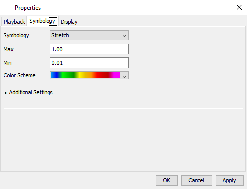
- View Incremental Precipitation and Air Temperature spatial results for the Jan97_interpolatedGrid_Bias simulation. Go to the Spatial Results toolbar and select Incremental Precipitation from the drop down menu. Open the Properties editor. As shown below, change the symbology to the Stretch option and enter a max upper limit of 1.0 inches. Click Apply and OK.
Drag the animation button to January 2, 1997 at 20:15 as shown in the figure below. You should see precipitation depths vary from about 1 inch (from 19:15 through 20:15, one hour accumulation) at the highest elevations to 0.25 inches at the watershed outlet.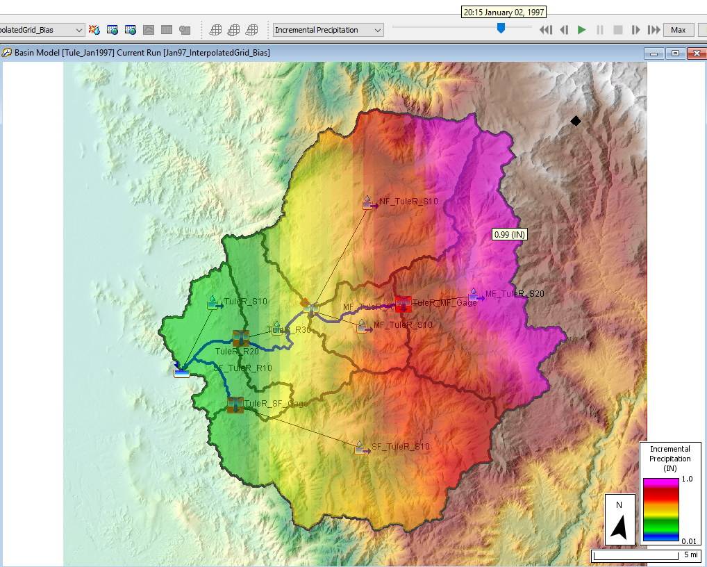
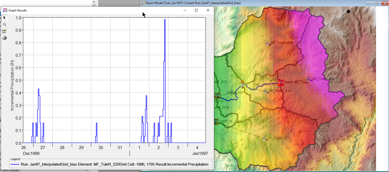
- You can right click on any location within the watershed to see a time-series plot of precipitation for the selected grid cell as shown below.
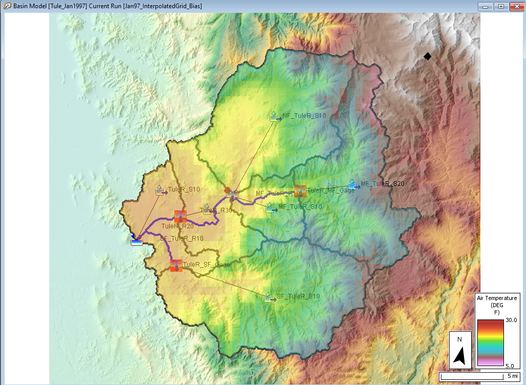
- As shown in the figure below, you can visualize the interpolated temperature as well. This figure was generated by setting the maximum display to 30 degrees F and minimum to 5 degrees F and clicking the Min button in the animation toolbar.
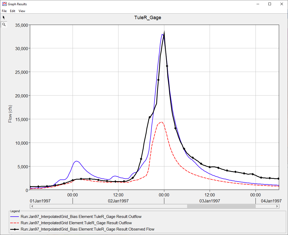
- Finally, compare the computed hydrograph at the TuleR_Gage junction element. As shown in the figure below, the simulation that used the bias precipitation grid to scale interpolated precipitation computed improved results. This is because the precipitation bias grid added precipitation volume that was not captured by the lone precipitation gage. Using a precipitation bias grid will be valuable for those applications where precipitation gages do not capture the spatial variability of precipitation, especially in those cases where precipitation was larger in orographically enhanced areas with no precipitation gages.