Download PDF
Download page Applying the Ensemble Compute to Flood Forecasting.
Applying the Ensemble Compute to Flood Forecasting
Last Modified: 2024-10-02 13:54:17.353
This tutorial demonstrates the new Ensemble Analysis compute option in HEC-HMS applied to a forecasting application.
Software Version
HEC-HMS version 4.11 beta 3 was used to create this example. You can open the example project with HEC-HMS 4.11 beta 3 or a newer version.Project Files
Example HEC-HMS Project:
 Gallinas_Creek_postCompute.zip
Buffered Polygon of Total Watershed:
Introduction
There are a number of numerical forecast products that are available and can be used as boundary conditions for your HEC-HMS model. Recent tool development has streamlined the process of gathering meteorologic boundary conditions and formatting the data for model simulations. The Ensemble Analysis compute option is a valuable tool that can be used to run multiple simulations and extract information across all ensemble members. This example demonstrates how to gather multiple meteorologic forecasts apply the HEC-HMS Ensemble Analysis compute to simulate possible runoff scenarios.
Watershed
The Gallinas Creek watershed is located in Northern New Mexico. Gallinas Creek is a tributary of the Pecos River. An HEC-HMS model of the upper portion of the Gallinas Creek watershed was created in response to the Calf Canyon / Hermits Peak fires that burned over 300,000 acres in the Sangre de Cristo Mountains, including a significant portion of the Gallinas Creek watershed upstream of Las Vegas, NM.
The following figure shows the subbasin delineation defined for the watershed. Small subbasins, approximately 2 square miles each, were delineated in an effort to estimate debris and sediment from burned areas in the watershed. The red element in the figure is the Gallinas Creek near Montezuma USGS gage location, 08380500.

The modeling methods used include the SCS Curve Number, SCS transform , Linear Reservoir baseflow, and Muskingum-Cunge reach routing methods. These methods were selected for rapid estimation of pre and post fire flow and debris/sediment estimation. Within the Gallinas_Creek_PreFire basin model, parameters were estimated using physical properties of the watershed and soil/landuse information. The model was calibrated to an event in 2013 using hourly precipitation from the AORC gridded dataset. The following figure shows the model results for at the Gallinas Creek near Montezuma USGS gage. The Gallinas_Creek_PostFire basin model was created by copying the Gallinas_Creek_PreFire basin model and adjusting Curve Numbers and SCS lag times to reflect changes to the runoff response due to burned conditions.

The summer 2022 monsoon season saw a number of precipitation events fall over the watershed. Five different forecasted precipitation datasets were downloaded for a 2-day period on August 17, 2022. These datasets were applied to both the pre and post fire basin models. The Ensemble Analysis was used to visualize precipitation and flow from the various meteorology and basin model combinations.
Analysis Procedure
The following list identifies the steps followed in the analysis. The example project already includes all components described below.
- Download Forecast Meteorology Datasets
- Convert Forecast Meteorology Datasets to HEC-DSS Format
- Create Gridsets in the HEC-HMS Project
- Create Meteorologic Models in the HEC-HMS Project
- Create Simulation Runs for Forecast Meteorology Datasets
- Create Ensemble Analysis Simulations
- Analyze Results
Download Forecast Meteorology Datasets
The following table contains information about the five forecast datasets used in this example. Some datasets, like the North American Mesoscale Forecast System (NAM), represent results from a single multidimensional atmospheric model and others, like the National Blend of Model (NBM), include a mean estimate of future precipitation from processing an ensemble of multidimensional atmospheric models. Scripts were used to download the data files to a local computer. The scripts are contained in the table below.
| Precipitation Product | Link to Data Product Description | Script to Download |
|---|---|---|
| NAM Conus (12km) | https://nomads.ncep.noaa.gov | |
| The High Resolution Ensemble Forecast (HREF) Mean | https://nomads.ncep.noaa.gov | |
| HiresWindow (HIRES) | https://nomads.ncep.noaa.gov | |
| High-Resolution Rapid Refresh (HRRR) | https://nomads.ncep.noaa.gov | |
| National Blend of Models (NBM) | https://vlab.noaa.gov/web/mdl/nbm |
You can run the data retrieval scripts using the python command prompt. Python might be on your computer already as part of another program. I used the python installed as part of the ArcGIS Pro software on my computer. You can install python as a separate installation.
- You will need to create directories in C:\Temp to house the downloaded forecast datasets. For example, the C:\Temp\hrrr directory was already created on my computer.
- Open the Python Command Prompt.
- Type "python.exe C:\Temp\retrieve_hrrr.py" to run the script (make sure you point to where the script is located on your computer).
- As shown below, the script will create a folder using today's date and begin downloading files.

Convert Forecast Meteorology Datasets to HEC-DSS Format
The following section describes how the numerical model data was imported into a HEC-DSS File using the Gridded Data Import option in HEC-HMS.
- Go to the File | Import | Gridded Data | Importer menu option to open the Gridded Data Import tool.
- Select the gridded data files for one of the data products from the first task.
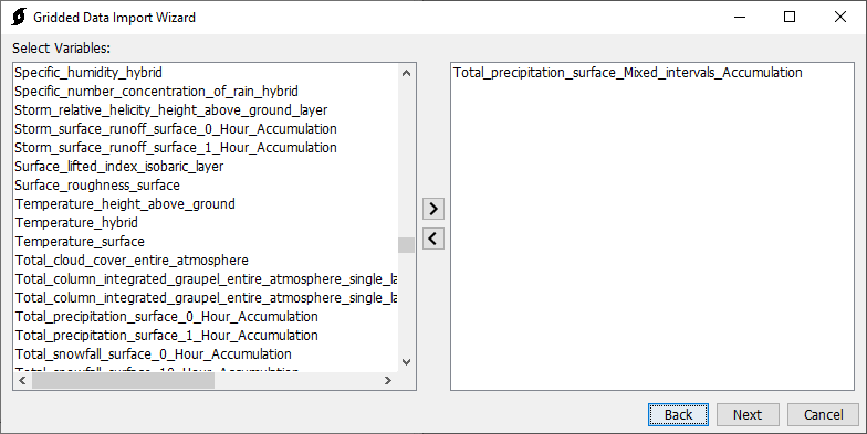
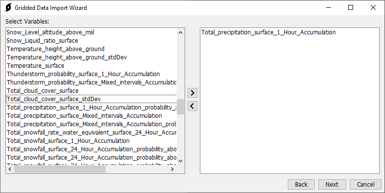
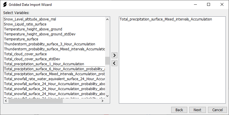
The table at the end of this section show which Variable to select when importing precipitation from the five datasets included in this example. Notice some of the precipitation datasets require that you run through the import process multiple times due to how the data is stored.
As shown in the following figure, select a clipping data source. Since these are national scale datasets, clipping the precipitation to the watershed extents greatly reduces file sizes. Choose a target projection. SHG was chosen in this example to match the discretization projection chosen in the basin model. The target cell size was left empty. The program does not resample the gridded data when the target cell size is left empty. The bilinear resampling method was selected.

- In the last step, you choose a destination DSS file, pathname parts, units, and data type. If importing precipitation, the Gridded Data Importer tool will automatically use PRECIPITATION for the C-part pathname, units of MM (for these five datasets) and set the data type to PER-CUM (you do not have to override the units and data type when importing precipitation using the datasets in this example).

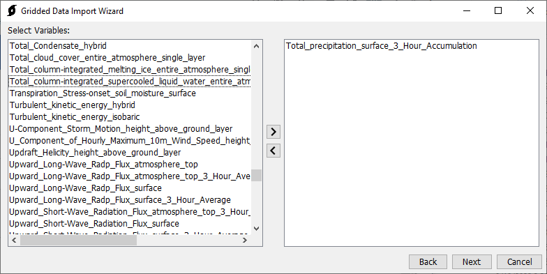
| Precipitation Product | Precipitation Variable | Notes |
|---|---|---|
| NAM Conus (12km) | Total_precipitation_surface_3_Hour_Accumulation
| For now, only select f03, f06 - f48 files when importing. A custom data converter is needed for importing NAM data. The grids are stored as accumulation over one, two and then three hours before resetting at the next three hour interval. |
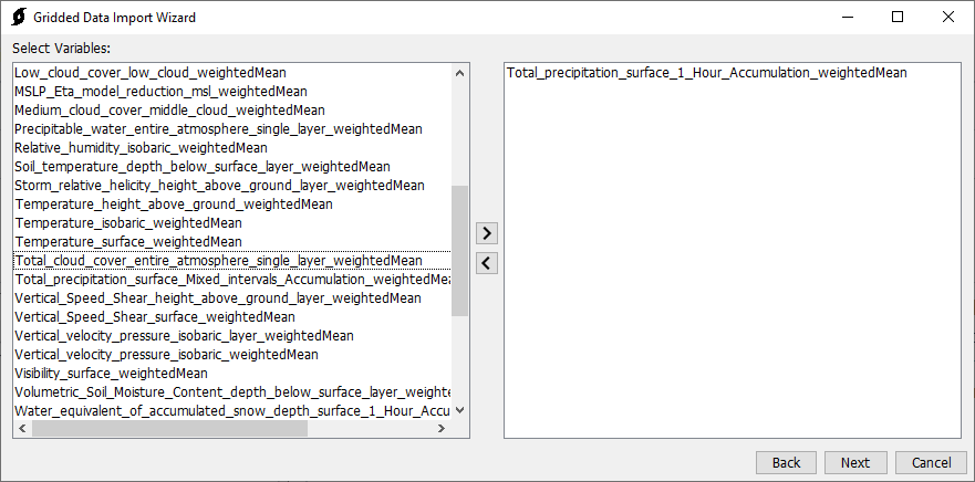
| The High Resolution Ensemble Forecast (HREF) Mean | Total_precipitation_surface_1_Hour_Accumulation_weightedMean
| 1-hour accumulated precipitation grids will be imported. |
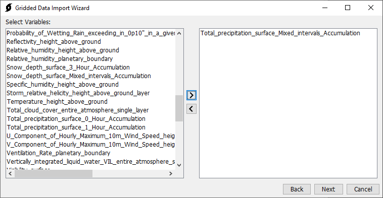
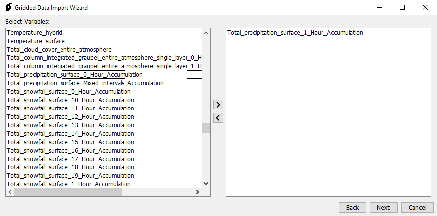
| HiresWindow (HIRES) | Total_precipitation_surface_1_Hour_Accumulation Total_precipitation_surface_Mixed_Intervals_Accumulation
| You must import both the 1-hour and mixed interval options in two separate import operations. The 1-hour import only imports the very first hour (you only select the first record). The mixed interval option imports the additional hourly forecast grids, and it also imports grids showing the accumulation from hour 0 to hour 1, 2, 3, and so on. After import, use HEC-DSSVue to delete the mixed interval records and only keep the regular interval hourly precipitation grids. |
| High-Resolution Rapid Refresh (HRRR) | Total_precipitation_surface_1_Hour_Accumulation Total_precipitation_surface_Mixed_Intervals_Accumulation
| You must import both the 1-hour and mixed interval options in two separate import operations. The 1-hour import only imports the very first hour (you only select the first record). The mixed interval option imports the additional hourly forecast grids, and it also imports grids showing the accumulation from hour 0 to hour 1, 2, 3, and so on. After import, use HEC-DSSVue to delete the mixed interval records and only keep the regular interval hourly precipitation grids. |
| National Blend of Models (NBM) | Total_precipitation_surface_1_Hour_Accumulation Total_precipitation_surface_Mixed_Intervals_Accumulation
| You need to break up the import into two separate import operations. Only select the first 36 records during the first import, these are hourly forecast grids. During the second import, select the remaining 3 hours grids. Choose mixed interval parameter. I noticed the 1-hour grid for 1100 - 1200 on the second day was missing. You might have to import a third round. |
Create Gridsets in the HEC-HMS Project
After the precipitation data was converted to gridded records in HEC-DSS files, gridded precipitation datasets were added to the HEC-HMS project and linked to the appropriate DSS files. The following steps describe how the precipitation gridsets were added to the HEC-HMS project. After adding these datasets to the project, you could continue to add more gridded records to the DSS files as more forecast data becomes available.
- Open the Grid Data Manager and create a Precipitation gridset. The gridset was named using the data source.
- Open the Component Editor for the precipitation gridset.
- As shown below, the Single Record HEC-DSS Data Sources selected, a DSS file selected, and a pathname was selected. This step was duplicated for all 5 forecast datasets.

Create Meteorologic Models in the HEC-HMS Project
A separate meteorologic model was configured for each of the 5 forecasted precipitation datasets. The following steps describe how meteorologic models were added to the HEC-HMS project.
- Open the Meteorologic Model Manager and add a new meteorologic model to the project.
- Set the precipitation method to gridded precipitation. The following figure shows the GriddedPrecip_HIRES meteorologic model. The meteorologic model was configured to use the Gridded Precipitation method.

- Open the Gridded Precipitation component editor and choose the appropriate precipitation gridset. The following figure shows the Gridded Precipitation component editor for the GriddedPrecip_HIRES meteorologic model. Notice the HIRES gridset is selected. A time shift of 6 hours was entered to shift the precipitation data to local time.

Create Simulation Runs for Forecast Meteorology Datasets
The following steps describe how simulation runs were created. The Ensemble Analysis compute requires existing simulation runs be created first before they can be added to an ensemble analysis.
- A Control Specifications was created for simulating the forecasts. The August2022 Control Specifications had a time window from 17 August 2022 - 19 August 2022. A simulation time-step of 30 minutes was selected.
- Simulation runs were created for each of the 5 forecast datasets using both the Pre and Post Fire basin models. The figure below shows all 10 simulation runs.

Create Ensemble Analysis Simulations
The following steps describe how the Ensemble Analysis simulations were created.
- Open the Ensemble Analysis manager from the Compute menu.
- Create a New Ensemble Analysis and make sure the Analysis Type is set to Simulation Runs.
- Two Ensemble Analyses were set up in the HEC-HMS project. One Ensemble Analysis simulation contained the simulations that were set up to use the Pre-Fire basin model and the different forecasted precipitation products. The other Ensemble Analysis simulation contained the Post-Fire basin model and the different forecasted precipitation products. The following figure shows the Component Editor for the Ensemble_PreFire ensemble analysis.

- One of the strengths of the ensemble compute is its ability to summarize important information. As shown below, the output Results editor was configured to save results for the PC10_Sub subbasin elements and the GallinasCreek_Montezuma junction element. The program will extract results from the individual ensemble members and save the selected results to the ensemble output file. For example, ensemble analysis results for the Ensemble_PreFire simulation are written to the Ensemble_PreFire.dss file located in the main project directory.

Analyze Results
The information in this section comes from the Results tab of the Watershed Explorer or from the ensemble compute DSS files. The following figure shows the available results from the two locations selected in the Results editor (see step 4 in the previous section).

Choose the Precipitation Total summary table for the PC10_Sub subbasin element. The following table identifies the forecasted precipitation product used within each of the 5 ensemble members. The HREF forecasted precipitation amount was the smallest with a total 2-day depth of 0.33 inches. The NAM forecasted precipitation amount was the largest with a total 2-day depth of 3.7 inches.
| Ensemble Member | Forecast Precipitation Dataset |
|---|---|
| 1 | HIRES |
| 2 | HREF |
| 3 | HRRR |
| 4 | NAM |
| 5 | NBM |

You can access the flow hydrographs at the GallinasCreek_Montezuma element from the results tab as well. You can also access the results from the output DSS file using HEC-DSSVue. The following figure shows the flow hydrographs for all 5 ensemble members contained in the Ensemble_PreFire DSS file. 