Download PDF
Download page Applying the New Frequency Analysis Compute Type.
Applying the New Frequency Analysis Compute Type
Intro
In this tutorial, you will learn how to apply new Frequency Analysis Compute option added to HEC-HMS 4.10. You will 1) use the Frequency Analysis Manager to create a new Frequency Analysis compute. You will then learn how to 2) add ordinates to the new compute. Frequency Analysis computes consolidate multiple simulation runs and summarize their results within a single table. Prior to the addition of the Frequency Analysis compute type, modelers would need to create and run a simulation for each frequency event. Results could only be viewed for the individual simulations. This tutorial demonstrates how the Frequency Analysis compute option removes the need for individual simulation runs, reducing analysis to a single simulation run that provides the results in a single table. This enhancement provides noticeable time savings while also making data management much easier.
Download the initial HEC-HMS project files - Initial_Indian_Creek_FA.zip
Watershed Location and Basics
The provided watershed–Indian Creek–has been divided into four subbasins, with a computation point at the Marion Junction. The initial watershed has been calibrated to the July 2014 event. The project contains Atlas 14 grids for 24 hour duration 2 year through 1000 year events. Also included are nine hypothetical storm meteorologic models that utilize the Atlas 14 grids. Finally, the Atlas 14 Region 3 Quarter 2 50% time pattern has been added to the model.
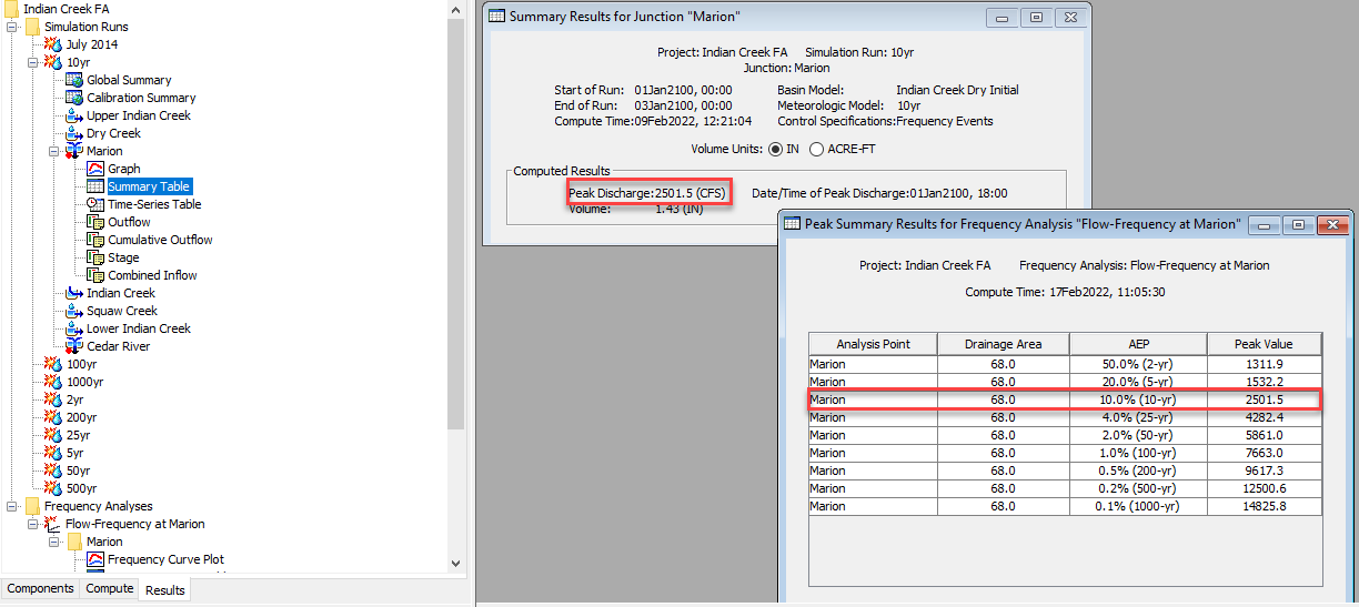
Existing simulation runs include a calibration simulation for the July 2014 event, as well as simulation runs for each of the nine frequency events. This initial watershed represents what would be the final results when modeling frequency events prior to the addition of the Frequency Analysis compute type.
Using the Frequency Analysis Compute
The Frequency Analysis Compute feature provides a convenient method of combining multiple computes into a single compute while also providing the benefit of consolidating the results of the multiple computes.
- Click Compute | Frequency Analysis Manager.
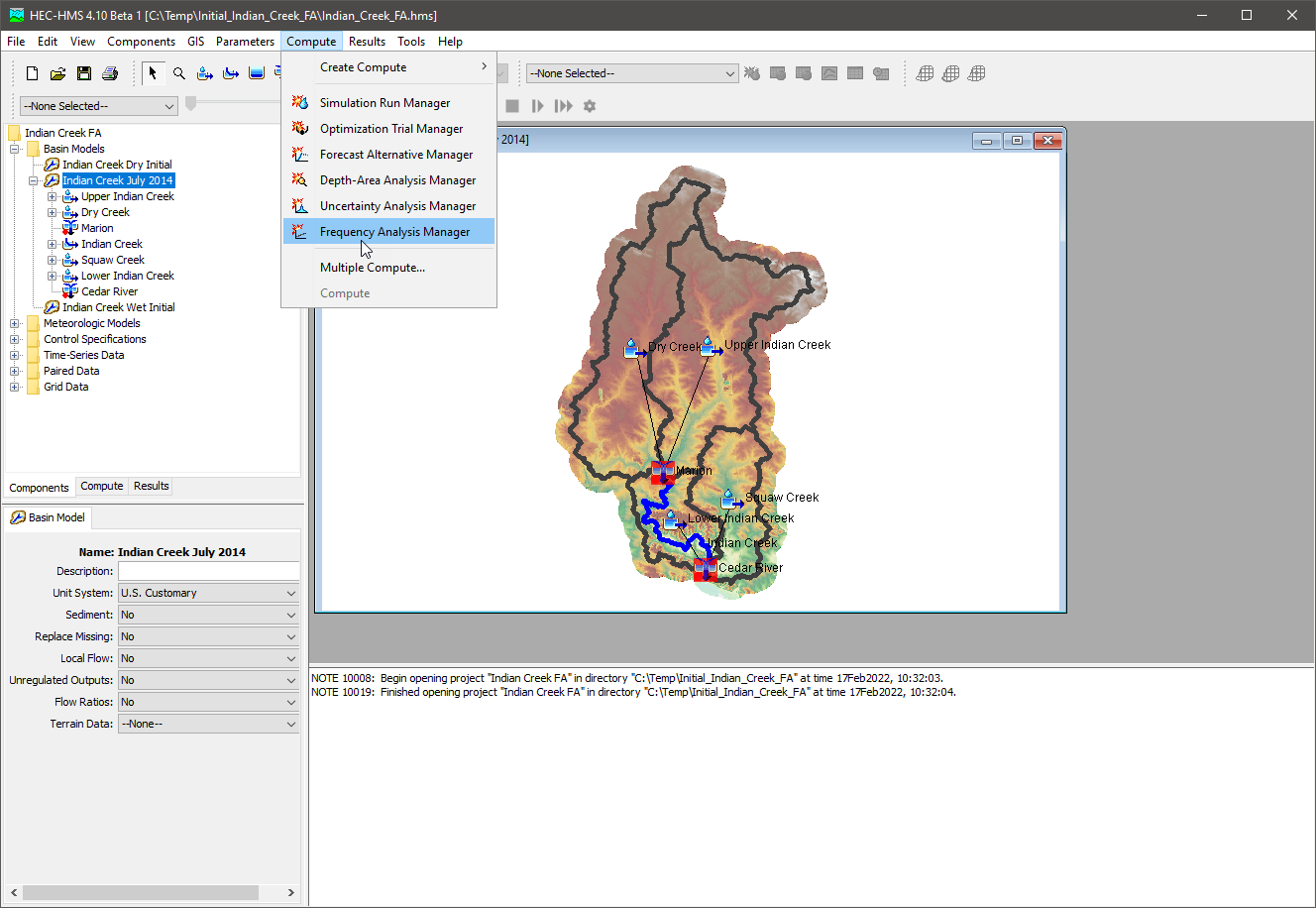
- In the Frequency Analysis Manager, click the New button.
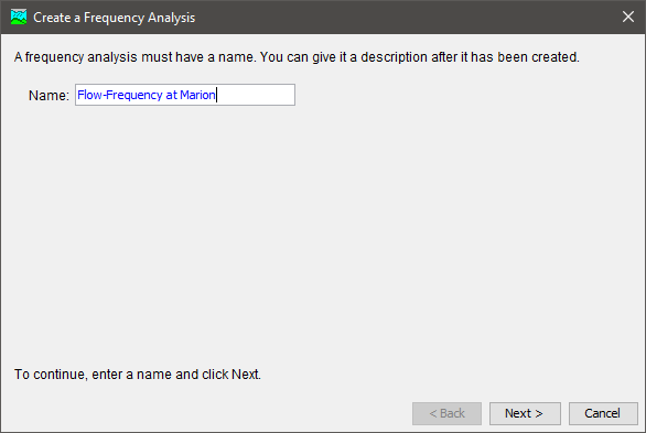
- Name the new Frequency Analysis compute Flow-Frequency at Marion, then click the Next button. Click the Finish button to complete the creation of the new compute type.
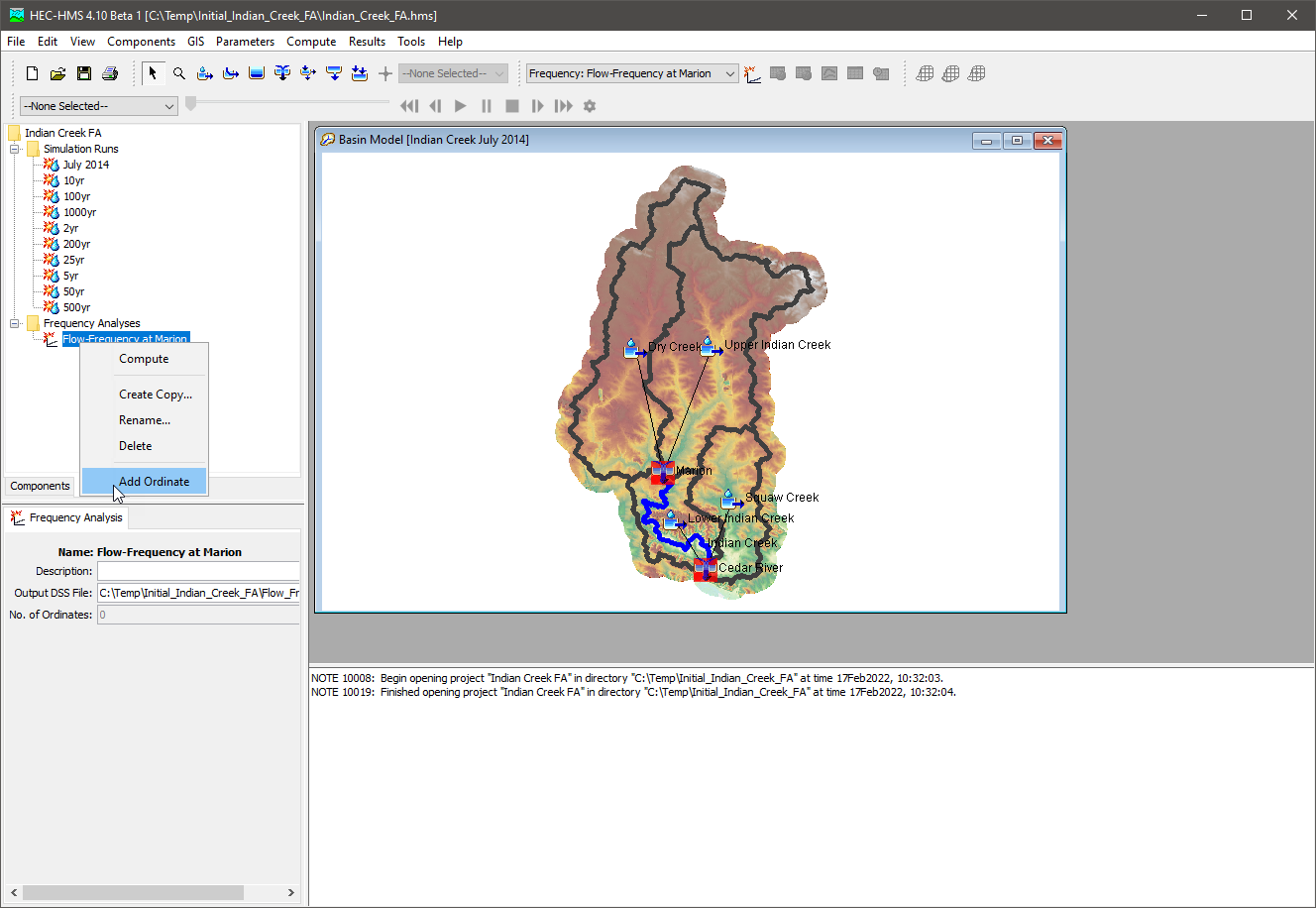
- Navigate to the Compute tab. A new Frequency Analysis folder has been added to the tree. Expand the folder and right click on Flow-Frequency at Marion, then click Add Ordinate to add the first ordinate.
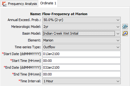
- Fill in the parameters for Ordinate 1 as shown in the figure below. Set the Annual Exceedance Probability to the 50.0% (2-yr) event. This ordinate will use Indian Creek Wet Initial for the Basin Model and the 2yr meteorologic model. Choose Marion as the element and Outflow as the time-series type. Set the start date to 01Jan2100 and start time to 00:00. Set the end date to 03Jan2100 and end time to 00:00. Finally, the simulation time interval should be set to 1 Hour.
- Create Ordinate 2 by right clicking on Ordinate 1 in the tree and selecting Copy Ordinate. Change the selected Annual Exceedance Probability to the 20.0% (5-yr) event and choose the 5yr Meteorologic Model, and Indian Creek Dry Initial Basin Model. The remaining parameters will remain the same.
- Create 7 copies of Ordinate 2 (for a total of 9 Ordinates), changing the Annual Exceedance Probability and Meteorologic Model for each ordinate.
- Run the analysis by clicking the Compute button
 in the Compute Control bar. The Compute Progress dialog will open, showing the Ordinates being computed sequentially. Close the Progress dialog when the compute has finished.
 - View the results of the compute by clicking on the Results tab and expanding the Frequency Analyses | Flow-Frequency at Marion | Marion in the tree.
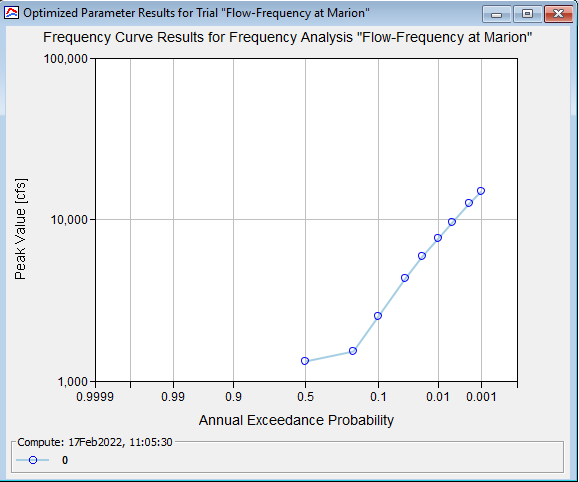
- First, open the Frequency Curve Plot. The Frequency Curve results for Frequency Analysis Flow-Frequency at Marion will open in the Map Window as shown below.
- Next, open the Frequency Curve Table. Notice that the Frequency Curve Table provides a summary of the computed flow at the Marion junction for all nine simulation events.
