Last Modified: 2023-11-22 17:37:10.501

Software Version

HEC-HMS version 4.12 beta 3 was used to create this tutorial. You will need to use HEC-HMS version 4.12 beta 3, or newer, to open the project files.

Project Files

Download the initial data files here:

maricopa_data.zip

Overview

This tutorial will guide you through the process of using various Maricopa County parameter estimation tools. The Maricopa Clark and S-Graph transform tools and the Green-Ampt loss tool became available in HEC-HMS version 4.9. More recently, in version 4.12, routing parameter estimation tools were added for the Muskingum, Kinematic Wave, Normal Depth, and Musking-Cunge methods. Each of these tools can be accessed by clicking Tools | Data | Maricopa. The Maricopa tools were designed specifically to accompany a standard work flow followed by Maricopa County water professionals.

Data

The Maricopa wizard tools will require several geo-spatial files and tabular CSV files as inputs. These include existing subbasin, reach, routing, longest flow path, soils, and land use shapefiles, as well as several landuse and soils tables in CSV format. These files are included in the zipped initial project files located above.

Creating a Geo-referenced Basin Model

Open HEC-HMS version 4.12 or later.
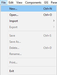
Create a new project by clicking File | New.
Specify the name, description, and location of the project as seen below. Select U.S. Customary as the default unit system.
Next, copy the GIS "maricopa_data.zip" folder to the "data" folder in the HEC-HMS project directory and unzip the files.
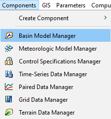
Now we need to create a basin model. Navigate to the basin model manager by selecting Components | Basin Model Manager.
Select New... and enter Maricopa as the name of the basin. Select Create.
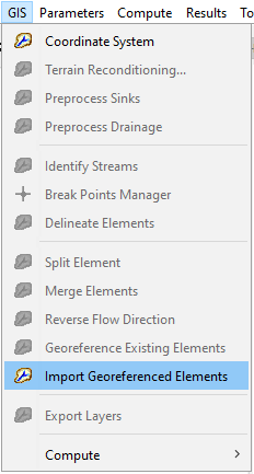
Now we need to import existing geo-referenced subbasins. Select the Maricopa basin model in the watershed explorer tree. Then select GIS | Import Georeferenced Elements.
In the first step of the wizard, select Subbasins. Click Next.
In the second step of the wizard, select the existing subbasins shapefile from the "data/maricopa_data" folder. Click Next.
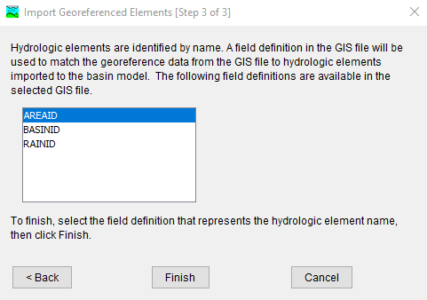
In the third step of the wizard, select AREAID as the field definition that represents the subbasin name. Click Finish.
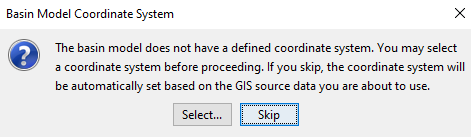
A popup will appear that prompts the user to specify a basin model coordinate system. Click Skip to use the projected coordinate system of the subbasin shapefile.
Now that we have a geo-referenced basin model, we need to change the transform method to Clark Unit Hydrograph. Click Parameters | Transform | Change Method...
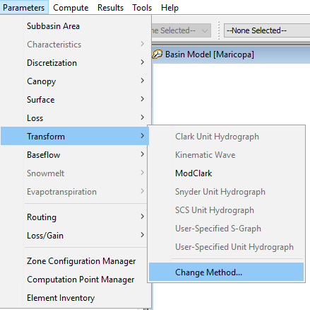
Click Yes to confirm that you wish to change methods. Select Clark Unit Hydrograph: Maricopa County AZ USA in the Method: dropdown box. Click Change.

HEC-HMS v4.12 Feature

In previous version of HEC-HMS, it was not possible to select the various Clark Unit Hydrograph sub-types (Standard, Variable Parameter, or Maricopa County AZ USA) from within the global editor. The sub-type had to be selected individually via the component editor for each subbasin which could be time-consuming. Starting in HEC-HMS v4.12, the sub-types for both Clark Unit Hydrograph and for User-Specified S-Graph can rapidly be set for all subbasin elements via the global editor.
To demonstrate the routing parameter estimation tools, a reach element is necessary. In a similar fashion to importing geo-referenced subbasins in steps 7 through 10 above, now let's import a geo-referenced reach element. Select GIS | Import Georeferenced Elements. This time, select Reaches as the element type. For the file, select the existing reach shapefile in the "data/maricopa_data" folder. Select name as the text attribute field. You should now have a geo-referenced basin model with three subbasin elements and one reach element.
Now let's connect the geo-referenced elements. To catch a sneak peak of what we hope to acheive after completing the next few steps, see the figure under step 19 below. First, we will need to create a junction element at the outlets of subbasin 010010 and 010005. Select the Junction Creation Tool and then, in the map pane, click near the outlets of the two uppermost subbasins. You can leave the name of the new junction element to the default entry of Junction-1.
In the watershed explorer, select the 010010 subbasin to open the subbasin component editor. For the Downstream selection, change it from None to Junction-1.
Now do the same for the 010005 subbasin, connecting it to Junction-1. Next, selection the Junction-1 element in the watershed explorer and change it's downstream connection from None to the CP1CP2 reach element.
As a last step, we need to create a sink element at the basin outlet that can accept the routed runoff from Junction-1 and the local runoff from subbasin 010015. Select the Sink Creation Tool and then, in the map pane, click near the downstream end of the CP1CP2 reach element. You can leave the name of the new sink element to the default entry of Sink-1.
Lastly, connect the 010015 subbasin and the CP1CP2 reach to the Sink-1 sink. The geo-referenced basin model with connected elements should look similar to the below figure.
The Maricopa Clark estimation tool requires longest flowpath characteristics. At this point, you can perform the steps necessary to compute subbasin characteristics in HEC-HMS (create/link a terrain model, perform steps on the GIS menu in HEC-HMS). Or you can go straight to the Maricopa Clark Wizard and provide a longest flowpath shapefile that contains an attribute field matching the subbasin names as well as attribute fields for upstream and downstream elevations in units of feet. For this tutorial, we will go straight to the Maricopa Clark Wizard to help us parameterize the associated transform parameters.

Applying the Maricopa Clark Parameter Estimation Tool

Navigate to the Maricopa Clark Tool by clicking Tools | Data | Maricopa | Transform | Clark...
The first step of the Maricopa Clark Wizard requires a basin model to be selected. Select the appropriate basin model and click Next.
The second step of the Maricopa Clark Wizard requires the user to select the land use shapefile, land use lookup table, and Kb lookup table. All the necessary files are located in the "data/maricopa_data/clark" folder. Furthermore, field names must be specified for two separate join operations to take place. The user must select the field names for the land use lookup table and land use shapefile join, and the user must also select the field names for the land use lookup table and Kb lookup table join. Lastly, the user needs to define the 'm' and 'b' lookup field names within the Kb table. Select the necessary inputs and click Next.
The third step of the Maricopa Clark Wizard allows for the user to use HEC-HMS subbasin characteristics in the Maricopa Clark calculations, or a longest flowpath shapefile can be specified instead.
For this example, we want to use an external shapefile for the Maricopa Clark calculations. Unselect the checkbox, and then select the longest flowpath shapefile and populate the appropriate fields for the subbasin id, upstream elevation, and downstream elevation. Note: using the longest flowpath shapefile option will override previously computed subbasin characteristics values, if they exist. Click Next to begin the computation.
Once the calculations are complete, the Clark Unit Hydrograph transform global editor will automatically be populated with Flowpath Length (MI), Adjusted Flowpath Slope (FT/MI) and Resistance Coefficient parameters. The user may choose to edit any of the calculated parameters in the global editor, or accept them as they are. Select Apply to save the parameters. This will save the values to the global editor and also populate the component editors for each of the subbasins. Save the project.
Additionally, HEC-HMS will output intermediate calculations as notes in the message console.

Applying the Maricopa S-Graph Parameter Estimation Tool

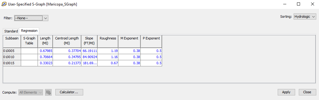
Similar to the Clark Parameter Estimation tool outlined above, a Maricopa S-Graph Parameter Estimation tool exists for the S-Graph transform method. The data input files needed for this tool are located in the "data/maricopa_data/sgraph" folder. After completing each of the wizard steps, the S-Graph Global Editor will be parameterized as seen below.
Additionally, HEC-HMS will output intermediate calculations as notes in the message console.

Applying the Maricopa Green-Ampt Parameter Estimation Tool

Let's use the Maricopa Green-Ampt Tool to calculate and populate loss and canopy parameters for the Maricopa basin model.
Select the basin Maricopa in the watershed explorer tree and click Parameters | Loss | Change Method...
Click Yes to confirm that you wish to change methods. Select Green and Ampt in the Method: dropdown box. Click Change.
Click Parameters | Canopy | Change Method...
Click Yes to confirm that you wish to change methods. Select Simple Canopy in the Method: dropdown box. Click Change. Save the project.
Navigate to the Maricopa Green-Ampt Tool by clicking Tools | Data | Maricopa | Loss | Green-Ampt...
The first step of the Maricopa Green-Ampt Wizard requires a basin model to be selected. Select the Maricopa basin model and click Next.
The second step of the wizard requires a landuse shapefile, landuse lookup table, soils shapefile, soils lookup table, and bare ground hydraulic conductivity (XKSAT) lookup table to be selected. All the necessary files are located in the "data/maricopa_data/green_ampt" folder. Select the necessary inputs and click Next.
The third step of the wizard involves defining the fields that will be used to join the landuse shapefile and landuse lookup table, as well as the soils shapefile and the soils lookup table. Specify the join fields and click Next.
The fourth and final step of the wizard involves matching various input parameters to their field names in the three lookup tables (landuse, soils, and hydraulic conductivity). Match the parameters to their field names in the lookup tables as seen below. If the header names in each of the three input tables follows the normal Maricopa convention, the dropdown menus should default to the correct selections. Click Next.
Once the calculations are complete, the Green and Ampt loss global editor will automatically be populated with Initial Type, Initial Deficit, Suction, Conductivity, and Percent Impervious parameters. The user may choose to edit any of the calculated parameters in the global editor, or accept them as they are. Select Apply to save the loss parameters.
Select Close to exit the Green and Ampt global editor. The Simple Canopy global editor should now be visible with calculated estimates for Max Storage. The user may choose to edit any of the calculated parameters in the global editor, or accept them as they are. Select Apply to save the canopy parameters.
Select Close to exit the Simple Canopy global editor. Save the project.
Additionally, HEC-HMS will output intermediate calculations as notes in the message console.

Applying the Maricopa Routing Parameter Estimation Tools

There are four routing methods that have parameter estimation tools (Muskingum-Cunge, Normal Depth, Kinematic Wave, and Muskingum). For this example, we will use the Muskingum-Cunge parameter estimation tool.

First, let's change the routing method in the existing Maricopa basin model to Muskingum-Cunge. Select the Maricopa basin model in the watershed explorer. Then select Parameters | Routing | Change method... Click Yes to confirm that you wish to change methods. Select Muskingum-Cunge in the Method: dropdown box. Click Change.
Navigate to the Muskingum-Cunge Tool by clicking Tools | Data | Maricopa | Routing | Muskingum-Cunge...
The first step of the Maricopa Clark Wizard requires a basin model to be selected. Select the appropriate basin model and click Next.
The second step of the Maricopa Muskingum-Cunge Wizard requires the user to select a Muskingum-Cunge routing shapefile. Choose the "Routing_Muskingum_Cunge_RC.shp" file located in the "data/maricopa_data/routing" folder. Furthermore, the field name for Channel shape must be specified; choose Eight Point. Lastly, for the reach name field choose ID and for the manning's n field choose MAN.
Since Eight Point was previously selected for the channel shape, the third step of the Maricopa Muskingum-Cunge Wizard allows an option for the user to use shapefile attributes to create eight-point cross-sections. Leave this option selected and make sure the below fields are selected. Click Next.
For this example, we want to use the previously provided routing shapefile for the Maricopa Muskingum Cunge length and slope calculations (otherwise previously calculated reach delineations and characteristics values for length and slope in HEC-HMS could be used). Unselect the checkbox, and then select the upstream elevation field and downstream elevation field as seen below. Click Next to begin the computations and parameterizations.
Once the calculations are complete, the Muskingum-Cunge routing global editor will automatically be populated with Length, Slope, Manning's 'n', Shape, Left Manning's 'n', Right Manning's 'n' and 'Cross Section' parameters. The user may choose to edit any of the calculated parameters in the global editor, or accept them as they are. Select Apply to save the routing parameters.
Notice that a cross-section named after the routing element, "cp1cp2_eightpoint" was automatically created and selected in the global editor. To visualize the cross-section, navigate to the watershed explorer, and expand the Paired Data node, the Cross Sections node, and then select "cp1cp2_eightpoint". Select the Graph tab to see a plot of the paired data.

You may follow a similar workflow to experiment with the other three Maricopa routing parameter estimation tools in HEC-HMS. These include Normal Depth, Kinematic Wave, and Muskingum. Other routing shapefiles are provided in the "data/maricopa_data/routing" folder.

Project Files

Download the final HEC-HMS project files here:

Maricopa.zip

Download PDF

Applying the Maricopa County Parameter Estimation Tools