Download PDF
Download page Importing Gridded SCS Curve Number in HEC-HMS.
Importing Gridded SCS Curve Number in HEC-HMS
Overview
This tutorial will step through how to import and apply a gridded curve number dataset in HEC-HMS. The Curve Number (CN) method is a widely used procedure for estimating precipitation excess/loss that takes into effect land use and soil types. The CN procedures were empirically derived from studies of small agricultural watersheds. Most applications of the CN method lumps the CN value as an average of the subbasin or watershed. HEC-HMS allows the modeler to either apply a subbasin average CN value or use a gridded approach where different CN values can be applied on a grid cell basis. Each each grid cell within a subbasin receives its own precipitation and losses/excess are computed based on the grid cell's CN value. To utilize the gridded curve number method in HEC-HMS, the modeler is required to convert their gridded curve number raster into a gridded DSS record. In the past, the asc2DSS.exe tool was used to convert ascii format grids to gridded DSS records. Recent development in HEC tools allow the HEC-HMS modeler to convert gridded CN rasters from common GIS formats to the DSS format using HEC-Vortex.
This tutorial was tested using HEC-HMS beta 4.10 and requires the users to have access to this version of the software. We will use the Pilot Creek watershed (watershed located approximately 12 mile south of Knoxville, TN) for this tutorial. The tutorial assumes you have already created your gridded curve number raster in a GIS. This tutorial does not describe how to delineate a watershed or how to set up a gridded precipitation simulation. You must also know how to create an empty DSS file. The project and associated files can be downloaded here: PistolCreek_Tutorial.7z
Review and process raster grid file
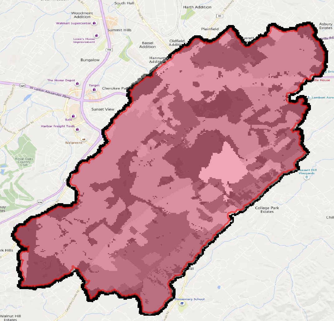
Make sure to review your gridded curve number raster file and that it overlaps your delineated watershed. You can find the CN raster file and watershed shapefile in the gis folder in the project directory (\PistolCreek_Tutorial\gis\). You will get an error in HEC-HMS at the start of the simulation if the CN grid does not overlap the subbasin boundary. A good practice is to create a buffer of your watershed shapefile and clip the CN grid to the buffered watershed. You can use your choice of GIS software, such as QGIS or ArcMap/Pro. The figure below confirms the CN grid overlaps the watershed area.
If you do not have a watershed shapefile, you can easily export one in HEC-HMS by selecting on the GIS menu → Export Layers
The next step is to import the CN raster file to DSS.
- Open HEC-HMS and go to File | Import | Gridded Data | Importer to open the Gridded Data Import Wizard.
- In the first window, select the folder to the right and add the CNgrid.tif located in the gis folder of the project. Click Next to continue to the next screen.
- Double click on CNgrid under Select Variables and click Next.
- In the next screen, leave the Clipping Datasource blank since the .tif file has already been clipped. For Target wkt, select the image of a globe on the right and choose SHG as the projection. In the same window, select 50 as the Target cell size. Click Next.
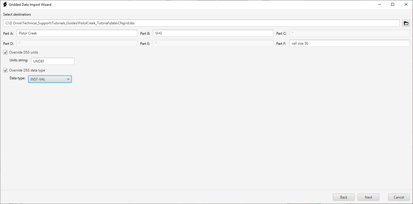
- In the Select Destination section, create a file named "CNgrid" and save the file in the data folder of the project directory (\PistolCreek_Tutorial\data\).
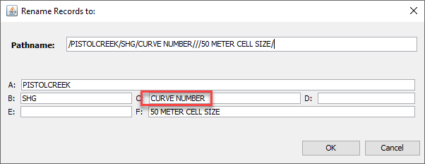
- Label the DSS paths as shown in the figure below. Check the Override DSS units and in the Units string type in UNDEF. Check the Override DSS data type and select INST-VAL as the Data-type.

This is a critical step. Units and data type must be set correctly for HEC-HMS to properly read the CN grid.
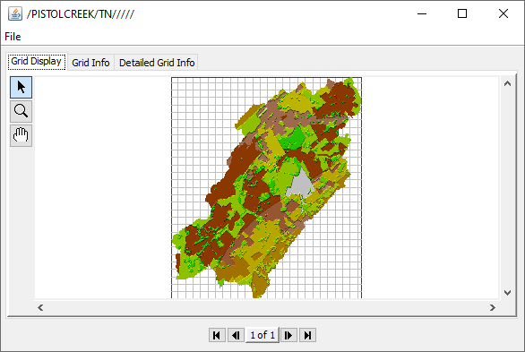
- Click next and the CN grid import should finish very quickly. Open your CNgrid.dss file and plot the CN grid to ensure the import process completed. You should see something like the image shown below in the Grid Display tab.
- In the Grid Info tab, check that the values match the figure below paying close attention to the Grid Type, Data Units, Data Type, and cell size.
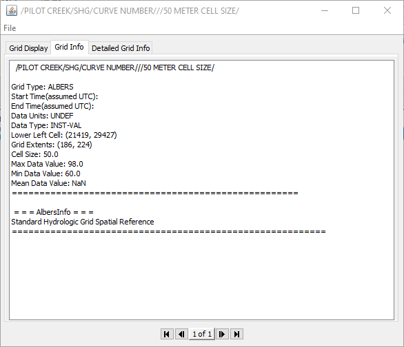
- Once those are confirmed, you will need to rename the Part C of the DSS record to CURVE NUMBER. This lets HEC-HMS know this grid is a curve number grid. Once these are checked, you are ready to import the grid into HEC-HMS.
You can select SHG or one of the UTM projections as well as any of the available cell sizes listed; however, your selected projection and cell size should be consistent with your discretization in the HEC-HMS model. This tutorial has the discretization set to SHG and 50 meters as the cell size. If the discretization has been set to 2000 meters, then the CN grid would need to be resampled to a 2000 meter cell size. If using gridded precipitation, the gridded precipitation projection must also be consistent with the CN grid and discretization. The precipitation grid size can be different from the CN grid cell size where you can have a 50 meter CN grid cell size and a 2000 meter precipitation grid size.
Adding DSS CN Grid to HEC-HMS
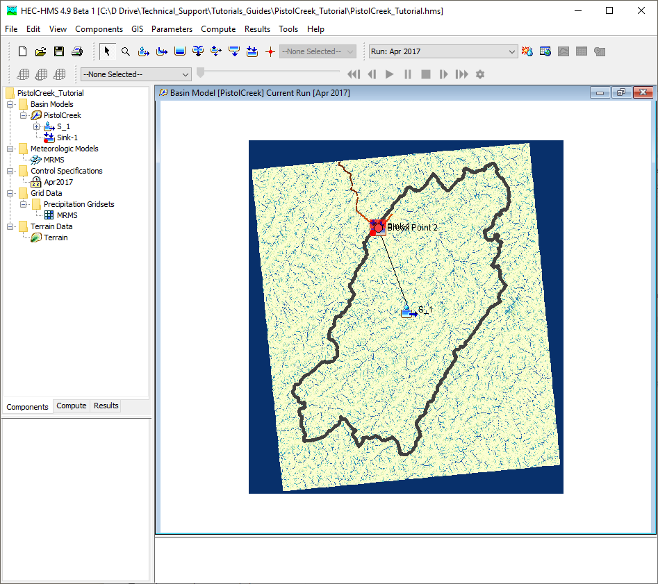
- Open the PistolCreek_Tutorial project in HEC-HMS 4.10. You should see a mostly complete project with a basin model, gridded precipitation meteorological model, control specification already set up.
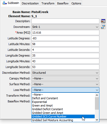
- Under the Basin Model, select Pistol Creek basin model. Check through all of the methods and parameters. You will notice that all of the methods and parameters have already been provided except for the Loss Method. Under the Loss Method, select Gridded SCS Curve Number.
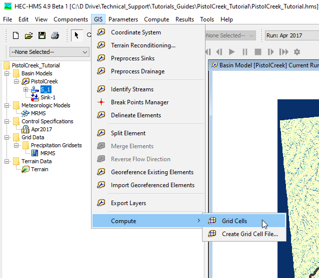
- In the Discretization tab, make sure the Projection and cell size is set to SHG and 50 meters. These values should be familiar to you since we set them during the CN grid import process. In the GIS menu, select Compute | Grid Cells to create your Discretization grid layer. You can view the created layer in the View | Map Layers editor. Make sure you check "Discretization".
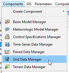
- Once you have your Discretization computed, add your newly created DSS CN grid file into the HEC-HMS project. This can be done by selecting Components | Grid Data Manager.
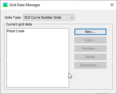
- Under Data Type, select SCS Curve Number Grids. Click "New" and type in Pistol Creek as the CN Grid name.
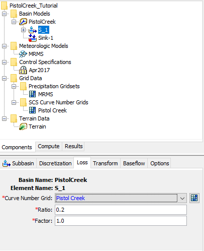
- Once you click OK, the SCS Curve Number Grids folder will appear under the Grid Data folder. Expand the SCS Curve Number Grids and select Pistol Creek. In the Component Editor, navigate to the location of your DSS file in the data folder (or wherever you saved your DSS file with the CN grid). In the DSS Pathname, select your CN grid record and save the project. In the Component Editor of your subbasin element, select the CN grid in the loss tab.
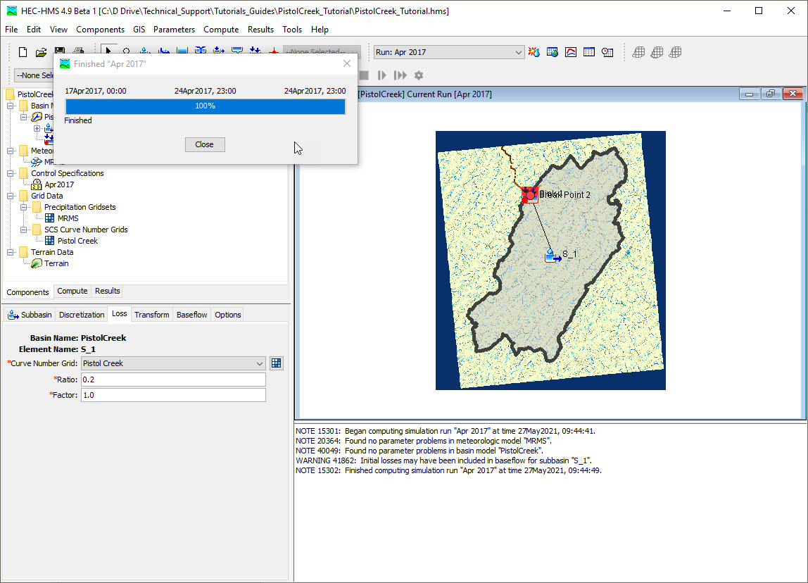
- Check that the CN grids were set up correctly by running a simulation. Head over to the compute tab and run the Apr 2017 simulation. The simulation should run to completion.
Although the Gridded Precipitation method is selected, non-gridded meteorological methods can also be used with the Gridded SCS Curve Number Loss method.
Setting up a Non-Gridded Curve Number Simulation
For comparison purposes, we are going to set up another basin model that uses the subbasin average Curve Number instead of the Curve Number grid.
- Create a copy of the PistonCreek basin model and name the copy PistolCreek_lumpedCN.
- Within the PistolCreek_lumpedCN basin model, change the loss method for the S_1 subbasin element to SCS Curve Number.
- We can use the GeoTiff file to estimate the basin average Curve Number.
- Open the Grid Data Manager and add a new SCS Curve Number Grid. Name the grid CN_GeoTIFF.
- As shown below, open the component editor for the CN_GeoTIFF grid and set the Data Source to GeoTIFF. Then choose the CNgrid.tif file located in the project's gis directory. Leave the units as None.

- Go back to the PistolCreek_lumpedCN basin model and select the Parameters | Loss | SCS Curve Number menu option to open the Curve Number global editor.
- Click the Calculator button the launch the parameter Expression Calculator.
- As shown below, choose the Curve Number parameter in the Field drop down. Then double click the CN_GeoTIFF grid to add it to the expression. Click the Calculate button. The program will compute the area average curve number value by intersecting the raster with the subbasin polygon.

- The computed Curve Number, 77.648, will automatically show up in the global editor and in the subbasin's component editor.

- Copy the Apr 2017 simulation run and name it Apr 2017 LumpedCN.
- Run the new simulation.
- The figure below shows computed outflow from the S_1 subbasin element for both the gridded and basin average Curve Number simulations.

Final Project Files