Download PDF
Download page HEC-HMS Example for Typical NRCS Applications.
HEC-HMS Example for Typical NRCS Applications
The following example was created using HEC-HMS version 4.10.
Background
The WinTR-20 software is a storm event (precipitation-runoff) model developed by the United States Department of Agriculture (USDA). The model can be used for event based flood modeling for water resource projects and uses hydrologic techniques developed by the Natural Resource Conservation Service (NRCS). HEC-HMS is another hydrologic modeling software that contains many different hydrologic methods and techniques, including methods from the NRCS. The information in this tutorial was originally developed for a WinTR-20 workshop example. As show in this tutorial, current HEC-HMS capabilities are available and provide similar workflow and results to the WinTR-20 software.
In this tutorial, you will:
- Create a new project
- Add hydrologic elements
- Connect the hydrologic elements
- Parameterize subbasin elements
- Parameterize reach elements
- Create the meteorologic models
- Configure and run simulations
- View results
HEC-HMS has additional capabilities not highlighted in this workshop and includes automated GIS tools, tools for processing Atlas 14 precipitation-frequency grids, and a Frequency-Analysis simulation type which can be used to build a flow frequency curve.
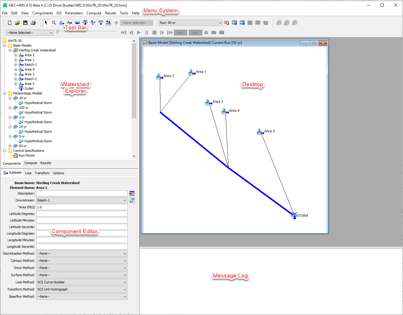
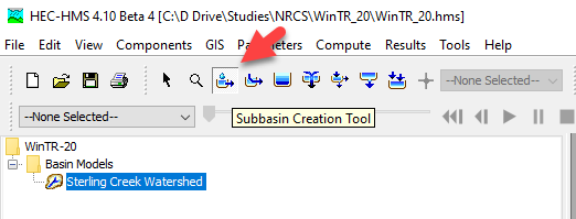
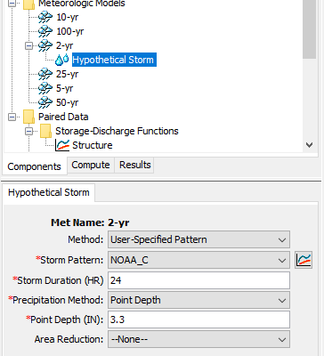
The following image shows the program screen in HEC-HMS with pertinent component names. These names will be helpful when navigating through the HEC-HMS Graphical User Interface.
Create a New Project
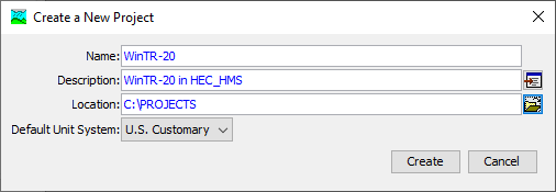
- Open HEC-HMS version 4.10 and create a new project by clicking on the File | New menu option. Name the project WinTR-20.
Add Hydrologic Elements
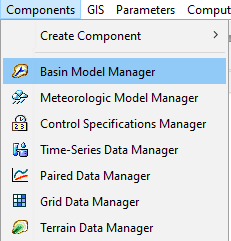
- Add a Basin Model to the project by clicking on the Components | Basin Model Manager menu option.
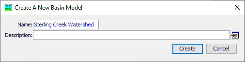
- In the Basin Model Manager window, click the New button and name the basin model Sterling Creek Watershed. Click the Create button.
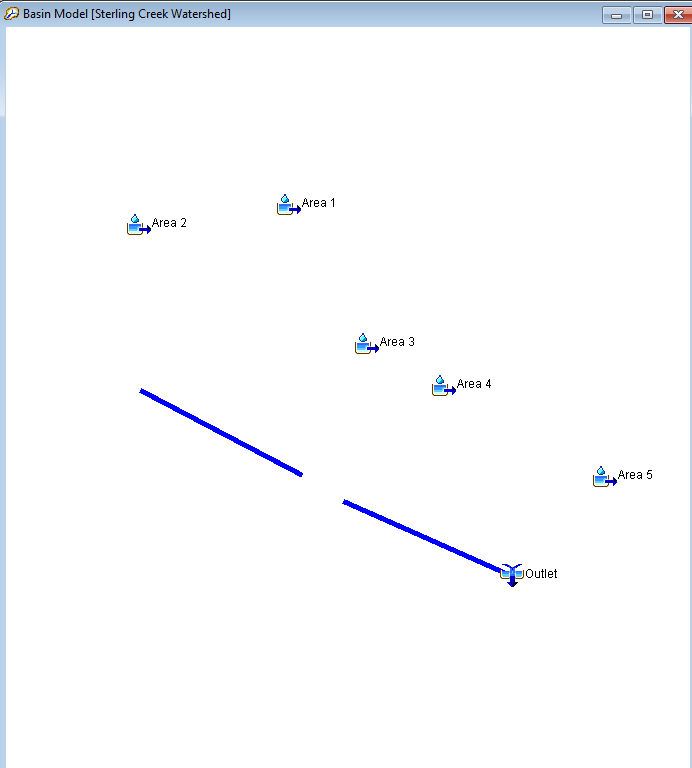
- You will see a Basin Models folder show up in the Watershed Explorer. Expand the folder and select the basin model you just created which allows you to create hydrologic elements. Select Subbasin Creation Tool and click in the basin model map area (located within the Desktop) to add a subbasin element.
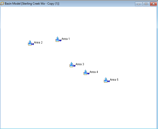
- Add four more subbasins to the basin model. You should have a total of five subbasin elements.
- Select the Reach Creation Tool to create a reach element. Click in the basin model map area and drag your mouse to your desired reach length. Click again to complete the reach. Name this Reach-1.
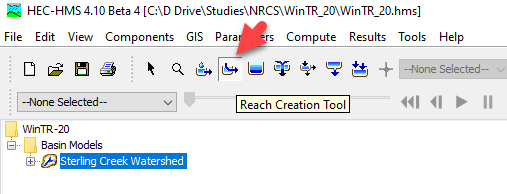
- Create one more reach, named Reach-2, for a total of two reaches.
- Select the Junction Creation Tool to add a junction element.
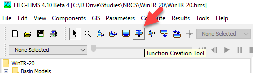
- Click the basin model map to add the junction. Name the Junction element Outlet. At this point, your basin model should have eight elements as shown below.
Connect the Hydrologic Elements
At this point, the hydrologic elements in the basin model are not connected.
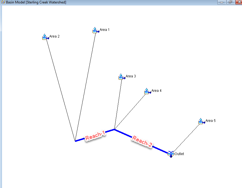
To connect elements, click on Area 1 in the Watershed Explorer. In Area 1's Component Editor, navigate to the Downstream dropdown and select Reach-1. Do the same thing for Area 2.

You can also connect elements by right clicking on the element in the basin model map, select Connect Downstream, and the click on the downstream element.
- Click on Reach-1 and in the Component Editor select Reach-2 as the Downstream element. Have Reach-2 connect to the Outlet.
- For Area 3 and Area 4, connect them to Reach-2.
- Have Area 5 connected to the Outlet. The final connections should look similar to the image below.
Parameterize Subbasins Elements
Once you have the elements connected, you can begin adding parameter values to the subbasin elements. The table below contains the relevant parameter values for each subbasin.
| Area 1 | Area 2 | Area 3 | Area 4 | Area 5 | |
|---|---|---|---|---|---|
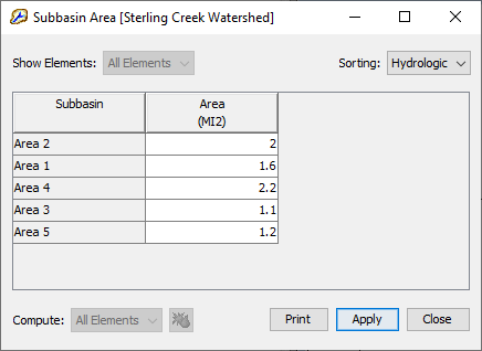
| Drainage Area (sq. mi.) | 1.6 | 2.0 | 1.1 | 2.2 | 1.2 |
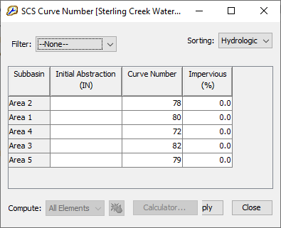
| Runoff Curve Number | 80 | 78 | 82 | 72 | 79 |
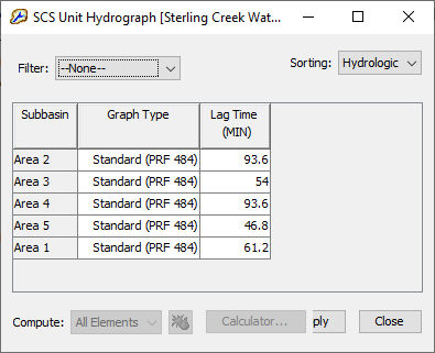
| Lag (min) | 61.2 | 93.6 | 54.0 | 93.6 | 46.8 |
- Baseflow will not be accounted for in this example. Click on the Sterling Creek Watershed Basin Model in the Watershed Explorer. This ensures the following changes will be made to al subbasins in the basin model. Turn off baseflow by selecting Parameters | Baseflow | Change Method menu option.
- In the Change Method window, select None as the Method. Click the Change button.
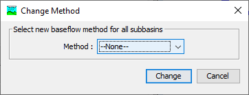
- In the Change Method window, select None as the Method. Click the Change button.
- In the Watershed Explorer, highlight the Sterling Creek Watershed Basin Model. Click the Parameters | Subbasin Area menu option (if you only see one subbasin, that means you had the element selected when opening the global editor). Enter the subbasin areas using the table below. Alternatively, you can also enter the area by clicking on each subbasin element and entering the Area in its Component Editor.
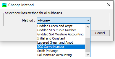
- Select the Parameters | Loss | Change Method menu option. Select Yes to change the method for all subbasins. Select SCS Curve Number method and click the Change button.
- Select the Parameters | Loss | SCS Curve Number menu option. In the Curve Number column, enter the curve numbers using the table below. Leaving the Initial Abstraction blank will result in HEC-HMS automatically calculating the initial loss as 0.2 times the potential retention, which is calculated from the curve number.
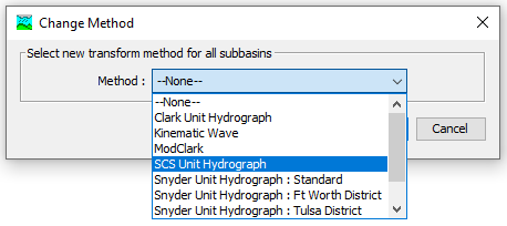
- Select the Parameters | Transform | Change Method menu option. Select Yes to change the method for all subbasins. Select the SCS Unit Hydrograph method and click the Change button.
- Select the Parameters | Transform | SCS Unit Hydrograph menu option. Enter the lag time values shown below. Leave the Graph Type as Standard (PRF 484).
Parameterize Reach Elements
- Select Reach-1 in the basin model map. In the Component Editor, change the Routing Method to Modified Puls.
- Select Components | Paired Data Manager to open the Paired Data Manager window. You will be creating two paired relationships: Storage-Discharge and Elevation-Storage.
- With Storage-Discharge selected as the Data Type, click the New button. Enter a name of Reach 1 S-D and click the Create button.
- Click on the Data Type drop down and select Elevation-Discharge. Select New and enter the name Reach 1 E-D.
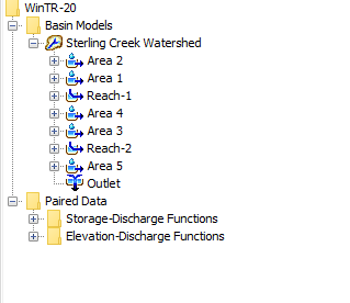
- Close out of the Paired Data Manager by clicking on the top right X. You will notice a Paired Data folder has been added to the Watershed Explorer. Expand the plus sign for the Paired Data folder to see a Storage-Discharge Functions and Elevation-Discharge Functions folders.
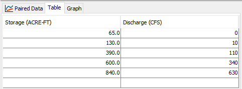
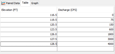
- Expand the Storage-Discharge Functions folder and click on the Reach 1 S-D paired data. In the Component Editor, click on the Table Tab to enter values using the table below.
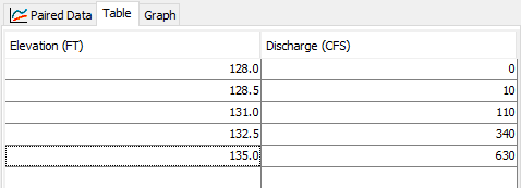
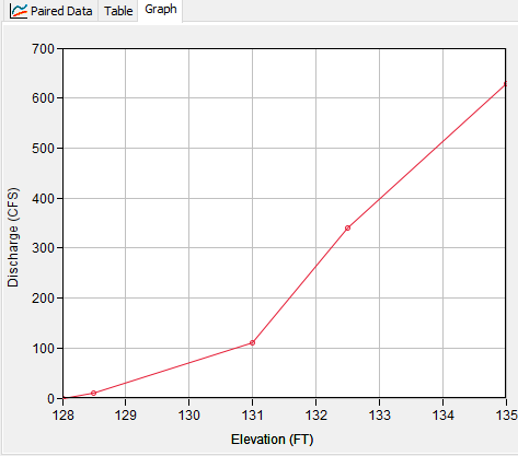
- Move onto the Elevation-Discharge Functions folder and click on the Reach 1 E-D paired data. In the Component Editor, click on the Table tab to enter values using the table below.
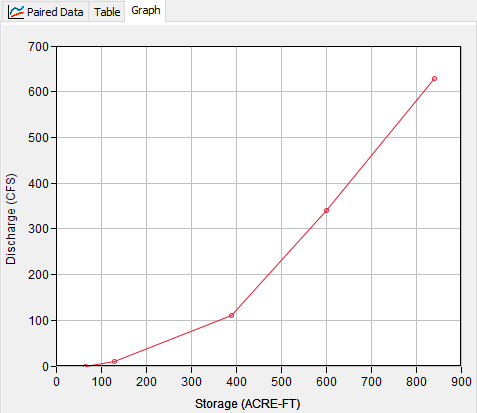
- You can also view the paired data relationship in a graph by selecting the Graph tab on either function.
- Click on Reach-1 either through the basin model map or Watershed Explorer.
- In the Component Editor, click the Routing tab and select the paired data for the Stor-Dis Function and Ele-Dis Function. Leave the Initial Type as Discharge=Inflow and Subreaches to 1.
- Select Reach-2 in the basin model map. In the Component Editor, change the Routing Method to Muskingum-Cunge.
- Navigate to the Components | Paired Data Manager menu to open the Paired Data Manager window again. Create a new paired data relationship for Elevation-Discharge, Elevation-Area Function and Elevation-Width and name the relationships Reach 2 E-D, Reach 2 E-A, and Reach 2 E-W, respectively.
- Expand the Elevation-Discharge Functions folder. There should be two paired data functions, Reach 1 E-D and Reach 2 E-D. Click on Reach 2 E-D paired data. In the Component Editor, click on the Table tab to enter the Elevation vs Discharge relationship as shown below.
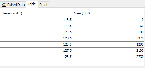
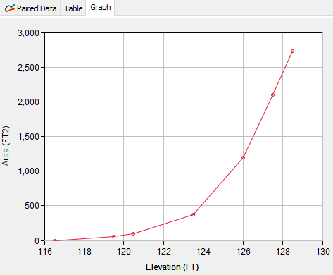
- Expand the Elevation-Area Functions folder and click on the Reach 2 E-A paired data. In the Paired Data tab, change the Units to FT:FT2. Navigate to the Table tab to enter the Elevation vs Area relationship as shown below.
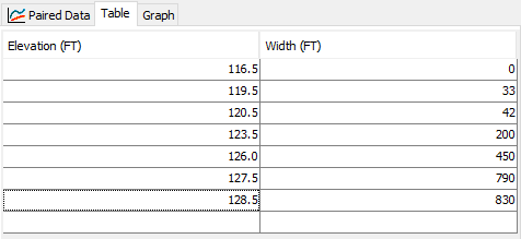
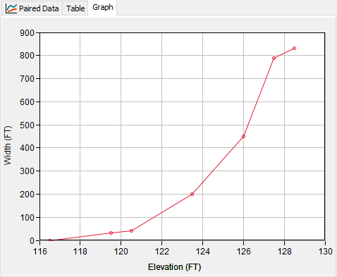
- Expand the Elevation-Width Functions folder and click on the Reach 2 E-W paired data. In the Component Editor, click on the Table tab to enter the Elevation vs Width relationship as shown below.
- You can also view the paired data relationship in a graph by selecting the Graph tab on either function.
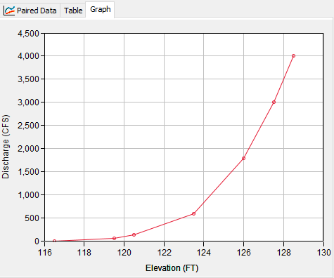
- Expand the Elevation-Discharge Functions folder. There should be two paired data functions, Reach 1 E-D and Reach 2 E-D. Click on Reach 2 E-D paired data. In the Component Editor, click on the Table tab to enter the Elevation vs Discharge relationship as shown below.
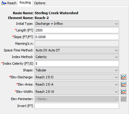
- Click on Reach-2 either through the basin model map or Watershed Explorer.
- In the Component Editor, click the Routing tab and change the Shape option to Tabular.
- Select the Reach 2 paired data relationship for Elev-Discharge, Elev-Area and Elev-Width.
- Leave the Initial Type as Discharge=Inflow.
- Set the Length to 2500 ft.
- Set the Slope to 0.0008.
- Change the Index Method to Celerity and set the Index Celerity (FT/S) to 5 ft/s.
Create Meteorological Models
Frequency based storms can be created in an HEC-HMS model using the Frequency Storm or Hypothetical Storm precipitation methods. The Hypothetical Storm precipitation method provides the ability to assign different storm durations and temporal patterns. Several default temporal patterns are available for the user to select (SCS Type 1, Type 1a, Type 2, and Type 3) as well as a User Defined option is available. More information on Hypothetical Storms is described in the User Manual. For this workshop, you will be selecting the User Defined option and entering in NOAA Atlas Type C distribution pattern. Download the spreadsheet NOAA_Dist_C.xlsx to obtain the NOAA temporal distribution for this example. The table below shows the basin average 24 hour frequency storm depths for the 2-yr to 100-yr storm events for the Sterling Creek Watershed.
| Storm Frequency | Rainfall depth (inches) |
|---|---|
| 2 year | 3.3 |
| 5 year | 4.2 |
| 10 year | 4.8 |
| 25 year | 5.9 |
| 50 year | 7.2 |
| 100 year | 8.4 |
- Create the NOAA Atlas Type C distribution pattern by navigating to Components | Paired Data menu and selecting the Percentage Curve Data Type. Click New in the Paired Data Manager window and name the paired data NOAA_C.
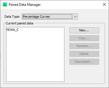
You should see a Percentage Curves folder in the Watershed Explorer. - Expand the Percentage Curves folder and click on NOAA_C paired data.
- Make sure the Data Source is selected as Manual Entry and navigate to the Table tab.
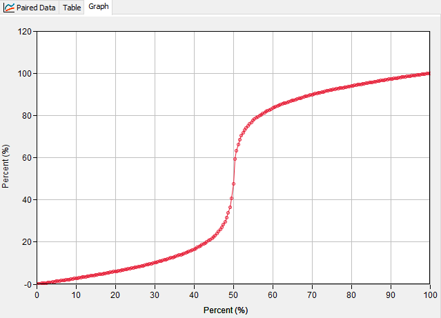
- Open the NOAA_Dist_C Excel spreadsheet and make sure the NOAA_C tab is open. Copy values in columns E and F starting (rows 3 through 243, the last values should be 100 for both columns).
Head back to your HEC-HMS project and paste the values into the Table. Click the Save button and Navigate to the Graph tab to view your temporal distribution.
NRCS Temporal Patterns
Below is an HEC-DSS file containing new NRCS temporal patterns. These patterns have been added to a DSS file using the paired data option. The x-axis is percent of the total storm duration (24 hours in most cases), and the y-axis the percent of the total storm depth. Use the following steps to use the records in the DSS file.
- Download the NRCSPercentageCurves.dss file to your HEC-HMS project's "data" folder.
- Create a new Percentage Curve in your HEC-HMS project (paired data).
- Set the Data Source to Data Storage System for the percentage curve.
- Select the correct DSS filename/path, and the correct DSS pathname.
HEC-DSS file with new NRCS temporal patters - NRCSPercentageCurves.dss
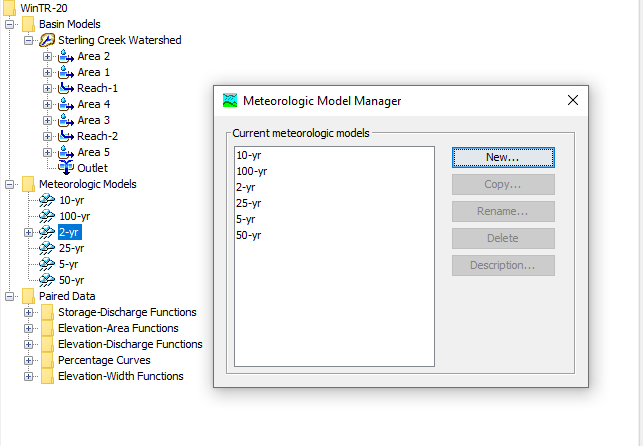
- Select the Components | Meteorological Model menu option. In the Meteorological Model Manager, click New and name the model 2-yr. A Meteorological Models folder will be created in the Watershed Explorer.
- Create five more met model and name them 5-yr, 10-yr, 25-yr, 50-yr and 100-yr. You should have a total of 6 meteorological models.
- Create five more met model and name them 5-yr, 10-yr, 25-yr, 50-yr and 100-yr. You should have a total of 6 meteorological models.
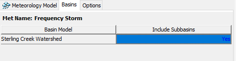
- Expand the Meteorological Model and click on the 2-yr meteorologic model. In the Component Editor, change the Precipitation method to Hypothetical Storm. Navigate to the Basins tab on the Component Editor and change the Include Subbasins to Yes for the Sterling Creek Watershed basin model.
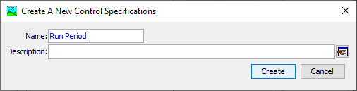
- Click on the Hypothetical Storm node for the 2-yr meteorologic model.
- In the Component Editor, change the Method to User-Specified Pattern.
- Select NOAA_C as the Storm Pattern.
- Enter 24 as the Storm Duration.
- Keep the Precipitation Method set to Point Depth and enter a value of 3.3 inches.
- Leave the Area Reduction set to None since the total drainage area at the outlet is less than 10 square miles.
- Repeat steps 4 and 5 again using the NOAA_C storm pattern for the other meteorological models (5-yr to 100-yr) and the frequency depths in the table at the beginning of this task.
Configure and Run Simulations
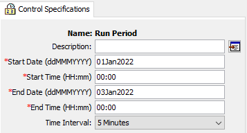
- Select the Components | Control Specifications Manager menu option. The Control Specifications Manager window will open. Click on New to create a new Control Specifications and provide the name Run Period.
A Control Specifications folder will appear on the Watershed Explorer. - Expand the Control Specifications folder in the Watershed Explorer and select on Run Period.
- Enter 01Jan2022 for the Start Date (ddMMMYYYY).
- Enter 00:00 for the Start Time (HH:mm).
- Enter 02Jan2022 for the End Date (ddMMMYYYY).
- Enter 24:00 for the End Time (HH:mm).
- Change the Time Interval as 5 Minutes.
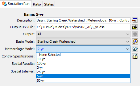
- At this point, we are ready to create our simulation. Select the Compute | Create Compute | Simulation Run menu option.
- Enter a name of 2-yr for the simulation run. Click Next.
- Select the Sterling Creek Watershed basin model.
- Select the 2-yr meteorological model.
- Select Run Period for the control specification.
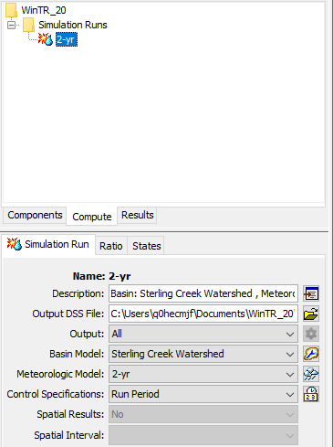
- On the bottom of the Watershed Explorer, click on the Compute tab
- Expand the Simulation Runs folder to see the 2-yr simulation you created.
- The Component Editor will show the selections you made for the Basin Model, Meteorological Model, and Control Specifications.
- Create the remaining simulation runs.
- Copy the 2-yr simulation by right clicking on it in the Watershed Explorer and selecting Create Copy. A Copy Simulation Run window will open.
- Change the name to 5-yr and select Copy.
- Select the 5-yr simulation run in the Watershed Explorer and change the Meteorological Model in the Component Editor to 5-yr.
- Repeat steps a and c for the remaining Meteorological Models (10-yr through 100-yr). You should have a total of six simulation runs.
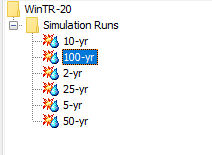
- To run the simulation, right click on 2-yr simulation run and select Compute. Do the same for the remaining simulation runs.
View Results
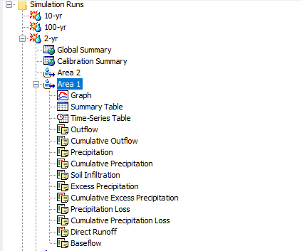
- On the bottom of the Watershed Explorer, click on the Results tab.
- Expand the Simulation Runs folder and click on the 2-yr simulation run. Results can be viewed for each element in the basin model.
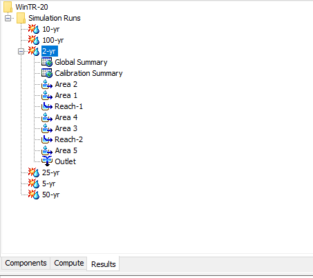
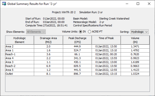
- Click on the Global Summary. This table provides the simulated peak flow information for each element.
- Select the Area 1 subbasin element. This provides detailed hydrologic information for Area 1.
- Click on the Graph. This provides a graph of the hyetograph and simulated runoff.
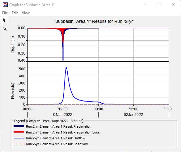
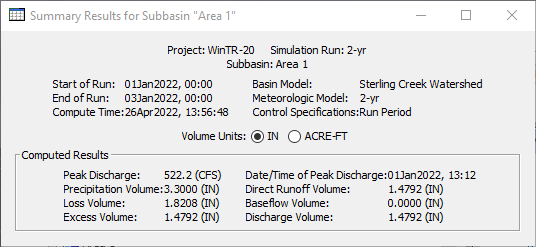
- Click on the Summary Table. This provides a summary of the computed hydrograph for Area 1.
- Click through the different options to view other results for Area 1.
- Review other Subbasin, Reach, and Junction elements.
- Click on the Graph. This provides a graph of the hyetograph and simulated runoff.
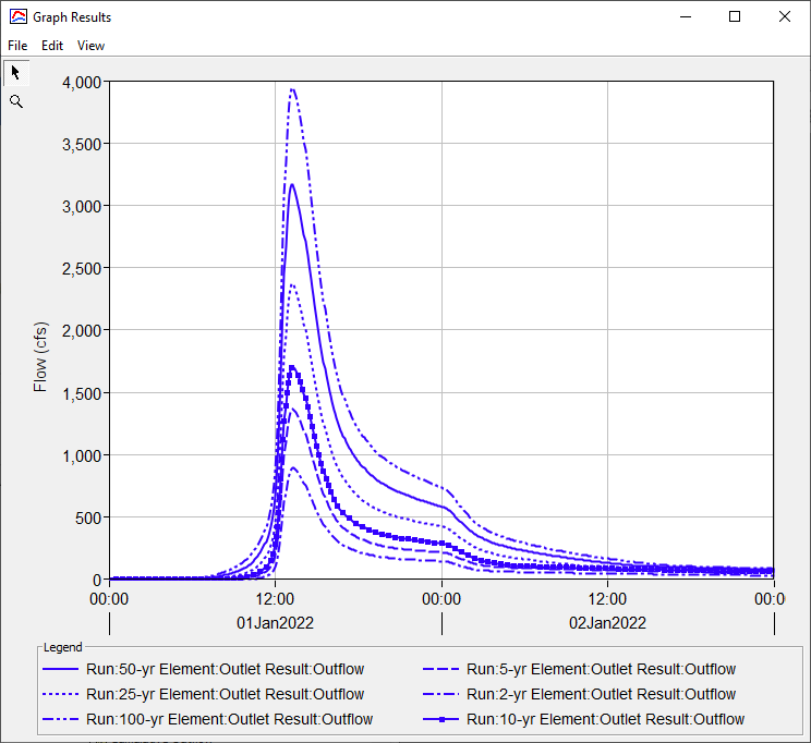
You can combine results from multiple simulations in one plot. Expand the results for all simulations, and expand results for the Outlet junction element. Hold down the control key and click on the Outflow time series from each simulation. Then click the plot button. You should see a plot similar to the one below.
- Click on the Global Summary. This table provides the simulated peak flow information for each element.
A couple of notes are listed below:
1) The unit hydrograph lag time might vary based on the precipitation and flow magnitude. We used only one basin model and the same SCS unit hydrograph lag parameter for all frequency based events. You can create separate basin models for each event and adjust the lag time as appropriate.
2) The loss parameters were kept constant for all simulations. It might be appropriate to vary initial condition for the magnitude of the storm event (based on the type of flood event, rain on snow vs tropical system).
3) HEC-HMS includes a Frequency Analysis simulation type. This simulation type is a nice way of organizing simulations and results for creating flow-frequency information. A Frequency Analysis was added to the project, results are shown below. 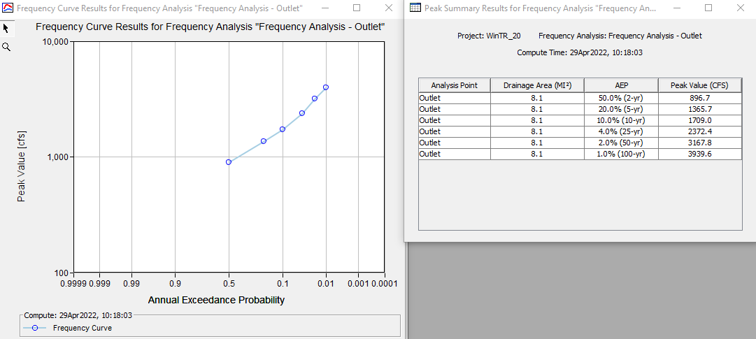
Download a final copy of the HEC-HMS model here - HEC-HMS Project
Compare Results with WinTR-20
The simulation results from HEC-HMS can be compared to the results from WinTR-20. Download the solutions file for WinTR-20 simulation workshop_1_solution.out.
The table below shows the 100-yr peak flow results computed from WinTR-20 and HEC-HMS. Notice that the peak flow values are close to each other.
| Element | Win20-TR Peak Flow (cfs) | HEC-HMS Peak Flow (cfs) |
|---|---|---|
| Area 1 | 2133 | 2149 |
| Area 2 | 1923 | 1962 |
| Area 3 | 1644 | 1652 |
| Area 4 | 1856 | 1894 |
| Area 5 | 1863 | 1861 |
| Reach 1 (downstream) | 605 | 606 |
| Reach 2 (downstream) | 2882 | 2903 |
| Outlet | 3972 | 3940 |
Question 1.) Why are the peak flow values not identical?
The differences are likely due to the different times steps between Win20-TR and HEC-HMS. Win20-TR computes a time increment as a function of the time of concentration using the equation:
| \Delta t=\frac{0.6 T_c}{((point number -1)-0.5)} |
where point number refers to the location of the peak along the dimensionless unit hydrograph. When estimating the time to peak, the time increment is set as the duration of excess rainfall. Although you can specify a time increment, the values are interpolated based on what is computed from the equation. For example, the 100 year storm event shows the following time increments for each subbasin
| Subbasin | Time Increment (hr) | Time Increment (min) |
|---|---|---|
| Area 1 | 0.107 | 6.42 |
| Area 2 | 0.164 | 9.84 |
| Area 3 | 0.095 | 5.70 |
| Area 4 | 0.164 | 9.84 |
| Area 5 | 0.082 | 4.92 |
HEC-HMS uses the time interval of 5 minutes which was set in the Control Specifications and is applied to all elements. Area 5, which has a time increment closest to 5 minutes, has a peak flow value that is nearly the same between the two models. You can change the time increment in HEC-HMS to 10 minutes and compare the outputs to Area 2 and Area 4 to confirm peak flows are similar.