Download PDF
Download page W3 - Applying the Linear Reservoir Baseflow Method.
W3 - Applying the Linear Reservoir Baseflow Method
Overview
In this workshop you will apply the HEC-HMS Linear Reservoir baseflow method to a modeling application. Initial parameter estimates will be estimated and the model will be calibrated through trial and error. HEC-HMS version 4.9 was used to created this workshop. You will need to use HEC-HMS version 4.9, or newer, to open the project files.
Download the Initial project files here - start_Linear_Reservoir_Workshop.zip
Background
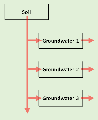
As implied by its name, the Linear Reservoir baseflow method uses one to three linear reservoirs (layers) to simulate the recession of baseflow after a storm event. Unlike the other baseflow methods, this method is guaranteed to conserve mass (i.e. precipitation losses = baseflow volume). The volume of infiltrated water is used as inflow to the Linear Reservoir method. Inflow can be partitioned to each layer in addition to deep aquifer recharge. As such, during periods of high infiltration, more baseflow will be generated. Conversely, during periods of little to no infiltration, less baseflow will be generated. When three groundwater reservoirs are used within this method, the system can be conceptualized as shown in the following figure.
Initial Parameter Estimates
- Open the Clark_UH_Workshop project and then open the Dec_1996_Jan_1997 Basin Model.
- Select the Dec_1996_Jan_1997 simulation run from the Compute toolbar.
- Press the Compute All Elements button to run the simulation.
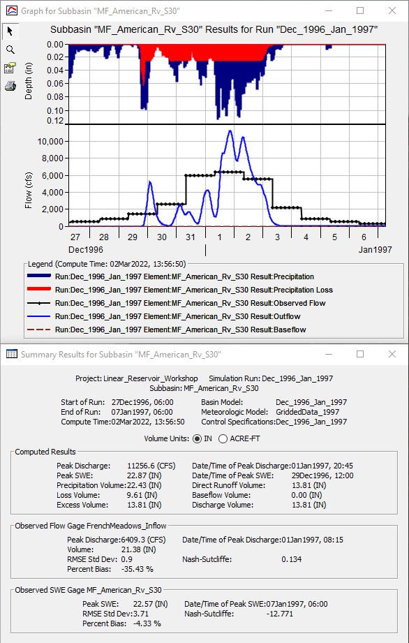
- View the result graph and summary table for the MF_American_Rv_S30 subbasin element, as shown in the following figure.
- Notice the volume of the computed hydrograph is significantly less than the observed hydrograph.
- No interflow or baseflow portions are included within the computed hydrograph.
- Leave the summary table and plot open so you can see results change as you add baseflow and modify baseflow parameters.
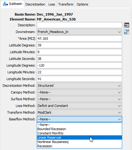
- Open the Component Editor for the MF_American_Rv_S30 subbasin element. Change the Baseflow Method from None to Linear Reservoir, as shown in the following figure.
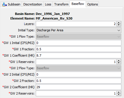
- Go to the Baseflow tab to enter Linear Reservoir parameters.
- Select 2 Reservoirs. We will use the Groundwater (GW) 1 layer to model faster responding interflow and GW 2 to model slower responding baseflow.
- Change the Initial Type to Discharge Per Area. Enter 0 CFS/MI2 for both GW 1 Initial and GW 2 Initial.
- Set the GW 1 Fraction to 0.5 and the GW 2 Fraction to 0.5. Initially, we are dividing all infiltrated precipitation equally between both GW 1 and GW 2 reservoirs.
- Set the GW 1 Coefficient so that it is 3 times larger than the ModClark Storage Coefficient (2.9 hours * 3 = 8.7 hours). Set the GW 2 Coefficient so that it is 10 times larger than the ModClark Storage Coefficient (2.9 hours * 10 = 29 hours).
- Leave the number of GW 1 Steps and GW 2 Steps at 1.
- Re-run the simulation and look at the results plot and summary table, as shown in the following figure.
- Notice baseflow in the plot and how the addition of baseflow to direct runoff results in an increase in the computed peak flow and volume.
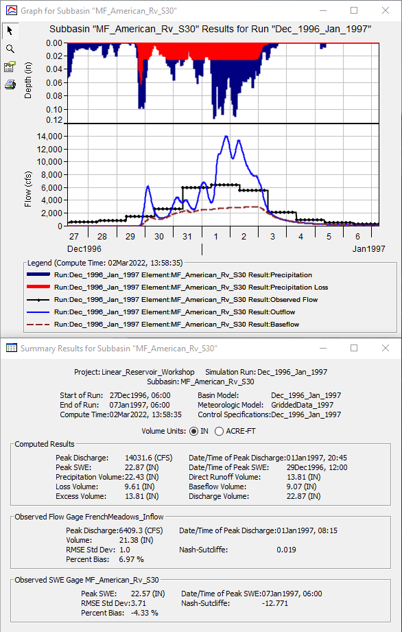
- Notice baseflow in the plot and how the addition of baseflow to direct runoff results in an increase in the computed peak flow and volume.
Calibrate the Model
- The easiest baseflow parameter modification to make is to set the initial baseflow at the beginning of the simulation so results match observed flow.
- For most applications, only use GW 2 to match observed flow at the beginning of the simulation.
- GW 1 typically represents faster responding interflow and leaves a watershed soon after a flood event.
- GW 2 typically represents the slower responding baseflow and is usually the only type of stream flow when there has been a longer period since a precipitation-runoff event.
- If you zoom into the plot, you will see the observed flow value is approximately 500 cfs at the start of the simulation.
- The drainage area for the subbasin is approximately 47 square miles
- Therefore, the initial GW 2 flow can be set by dividing 500 cfs by 47 square miles, which is approximately 10.6 cfs/sq mi. Change the GW 2 Initial value from 0 to 10.6 cfs/sq mi.
- Rerun the simulation. You should notice a close match in observed and computed flow at the beginning of the simulation, as shown in the following figure.
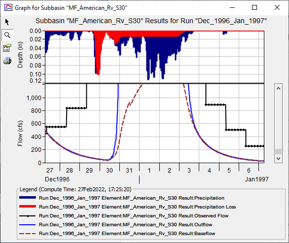
- The next step is to identify the parameters to adjust and understand their impact on computed results. Since the Linear Reservoir baseflow method conserves mass, loss parameters should be adjusted along with the baseflow parameters to improve model results.
- Change the Initial Deficit to 2.0 inches, and rerun the simulation.
- Notice the volume of baseflow and total discharge from the subbasin increased.
- Also, notice that the baseflow hydrograph now starts to rise on December 29th (approximately 24 hours earlier than the initial results indicated).
- Change the Constant Loss Rate to 0.15 in/hr and rerun the simulation.
- Notice the computed peak flow decreased. However, the volume of baseflow increased.
- This indicates that less surface runoff is generated while more baseflow is generated when increasing the constant loss rate
- Continue modifying parameters and noting the differences as each parameter is changed.
- Try increasing/decreasing the GW 1 Coefficient and GW 2 Coefficient.
- Try increasing the number of GW 1 Reservoirs and GW 2 Reservoirs.
- Try setting the GW 1 Fraction to 0.1 and the GW 2 Fraction to 0.9.
- Try setting the GW 1 Fraction to 0.1 and the GW 2 Fraction to 0.1.
- Continue adjusting the Deficit and Constant loss method and Linear Reservoir baseflow parameters to calibrate the model. Be sure you compute each time a parameter is modified so that you can observe the incremental changes to baseflow.
Questions:
Question 1. When using the Deficit and Constant loss method in combination with the Linear Reservoir baseflow method, which time series from the loss method are available for baseflow?
Within each subbasin element, water that infiltrates due to the constant loss rate contributes to baseflow. Water that is lost to satisfy the moisture deficit (i.e. initial deficit and any moisture deficit that is gained through evapotranspiration) DOES NOT contribute to baseflow.
Question 2. What advantages are realized by relating the Linear Reservoir groundwater coefficients to the Clark unit hydrograph parameters?
Clark unit hydrograph parameters can be estimated using physically-measurable characteristics. By relating these two processes using simple ratios, you can also estimate Linear Reservoir parameters using physically-measurable characteristics.
Another reason to relate the two processes is to reduce the complexity of parameterizing a basin model with many subbasins. Using ratios (i.e. 3 * R or 10* R) is a quick way to parameterize a model while linking parameters that are conceptually similar.
Similar processes that impact storage, attenuation, and timing of surface water also impact the response of interflow and baseflow. Interflow and baseflow happen throughout the watershed. Infiltrated water moves through the soil and then exfiltrates into a small channel. Once in the channel network, water flows in the stream network to the subbasin outlet. The path water takes after it exfiltrates into a channel is similar to the path direct runoff takes. The difference is that groundwater flow / baseflow spends a portion of the travel time in the soil, which is accounted for by increasing the baseflow coefficient or adding multiple linear reservoirs (steps).
However, it is not absolutely necessary to link the Linear Reservoir baseflow coefficients to the Clark unit hydrograph parameters. Other considerations (e.g. geological formations that significantly differ from surface features, etc) may also impact baseflow and should be considered when parameterizing the baseflow method.
Question 3. How do changes in the GW 1 and GW 2 Coefficients impact the baseflow hydrograph?
Increasing the GW 1 and GW 2 Coefficients will shift the baseflow hydrograph later in time. Conversely, decreasing these coefficients will shift the baseflow hydrograph sooner in time. In general, GW 1 should be used to simulate faster-responding interflow while GW 2 should be used to simulate slow-responding baseflow. Thus, GW 1 < GW 2. Also, keep in mind that interflow and/or baseflow should never respond faster than direct runoff, unless there is a physically-justifiable reason.
Modify GW 2 to match the receding limb of the observed hydrograph.
Question 4. How do changes in the number of GW 1 and GW 2 Reservoirs impact the baseflow hydrograph?
Increasing the number of GW 1 and GW 2 Reservoirs attenuates the baseflow hydrograph and shifts the baseflow peak downwards. Computationally, when multiple GW 1 Reservoirs are used, the outflow from the first GW 1 Reservoir is passed into the second GW 1 Reservoir, the outflow from the second GW 1 Reservoir is passed into the third GW 1 Reservoir, and so on and so forth.
Similar to increasing the GW 1 and GW 2 Coefficients, the number of reservoirs can be used to better match the receding limb of the observed hydrograph.
Question 5. How do changes in the GW 1 and GW 2 Fractions impact the baseflow hydrograph? How much water is lost to deep storage when the GW 1 and GW 2 Coefficients are set to 0.1 and 0.1?
The GW 1 and GW 2 Fractions are used to shift infiltrated water between groundwater layers.
When the GW 1 Fraction is set to 10% and the GW 2 Fraction is set to 90%, more infiltrated water goes to the slower-responding GW 2 linear reservoir (90 percent to the GW 2 reservoir vs. 10 percent going to the GW 1 linear reservoir).
In general, evenly dividing infiltrated water between the Linear Reservoir layers is a good place to start when calibrating the model.
The GW 1 and 2 Fractions can be used to remove water to a deep, non-contributing aquifer. The GW Fractions DO NOT have to sum to a value of 1. If the Fractions do not sum to 1, then the difference (i.e. 1 - sum of the GW Fractions) is lost to a deep aquifer and will not contribute to runoff from the subbasin. When each fraction is set to 0.1, 80% of the water that is infiltrated due to the constant rate is lost to deep storage.