Download PDF
Download page W6 - Applying the Variable Clark Unit Hydrograph Method.
W6 - Applying the Variable Clark Unit Hydrograph Method
Overview
In this workshop you will apply the HEC-HMS Variable Clark unit hydrograph method to a modeling application. Initial parameter estimates will be estimated using GIS information. HEC-HMS version 4.9 was used to created this workshop. You will need to use HEC-HMS version 4.9, or newer, to open the project files.
Download the initial project files here - start_Variable_Clark_Workshop.zip
Background
According to Sherman, the unit hydrograph of a watershed is “…the basin outflow resulting from one unit of direct runoff generated uniformly over the drainage area at a uniform rainfall rate during a specified period of rainfall duration” (Sherman, 1932). This implies that ordinates of any hydrograph resulting from a quantity of runoff-producing rainfall of unit duration would be equal to corresponding ordinates of a unit hydrograph for the same areal distribution of rainfall, multiplied by the ratio of rainfall excess values. However, due to differences in areal distributions of rainfall and hydraulic reactions between large and small precipitation events, the corresponding unit hydrographs have not been found to be equal, as implied by unit hydrograph theory (Minshall, 1960; Meyersohn, 2016). These realizations must also be combined with the fact that most precipitation events used when calibrating hydrologic models are normally much less intense than those used to design dams and other water resources infrastructure.
In an attempt to use conservative runoff parameters and counteract the inherent linearity of unit hydrograph theory, guidance has been followed within the U.S. Army Corps of Engineers (USACE) for approximately 50 years requiring the use of unit hydrograph peaking factors between 1.25 and 1.5 when simulating design storms (e.g. the Probable Maximum Precipitation, PMP) within dam safety studies (U.S. Army Corps of Engineers, 1991). This action shifts the resultant peak unit response at the location of interest upwards and earlier in time while maintaining the same runoff volume. These peaking factors are typically applied uniformly throughout time and space. The concept of peaking the unit response at a particular location is visualized within the following figure.

However, the applicability of these rules of thumb is not thoroughly analyzed within most dam safety studies. For instance, it is unknown whether a 25% peaking factor over or under-predicts the true unit hydrograph of a watershed in response to the PMP. Similarly, it is unknown whether a 50% peaking factor over or under-predicts the true unit hydrograph. Also, applying these peaking factors uniformly in time and space likely overpredicts the runoff response of a watershed during times of low excess precipitation rates (Bartles & Fleming, 2016). As an alternative, excess precipitation vs. Tc and R relationships can be used to simulate these effects in both spatially and temporally appropriate ways (Bartles, 2014; Bartles & Fleming, 2016). For example, only the subbasins of interest and most extreme periods of excess precipitation should be modified. The Variable Clark unit hydrograph method allows the user to make use of these excess precipitation vs. Tc and R relationships.
Review Clark Unit Hydrograph Parameter Estimation
Recall that separate regression equations were developed for time of concentration and watershed storage coefficient. The regression equations and techniques presented within the W2 - Applying the Clark/ModClark Unit Hydrograph Method workshop were used to estimate Clark unit hydrograph parameters for the study area.
Subbasin | L (mi) | DA (sq mi) | S1085 (ft/ft) | LSqrtDAS | RR | Tc (hr) | R (hr) |
|---|---|---|---|---|---|---|---|
| MF_American_Rv_S30 | 17.7 | 47.2 | 0.01937 | 875.3 | 0.04044 | 3.2 | 2.9 |
Review Clark Unit Hydrograph Calibration Results
Next, review the results of the Dec_1996_Jan_1997 simulation. Recall that the Clark unit hydrograph parameters were applied and calibrated within the W2 - Applying the Clark/ModClark Unit Hydrograph Method workshop.
- Open the Variable_Clark_Workshop project.
- Open the Dec_1996_Jan_1997 Basin Model.
- Select the MF_American_Rv_S30 subbasin element.
- Select the Dec_1996_Jan_1997 simulation run from the Compute toolbar,
 .
. - Press the Compute All Elements button,
 , to run the simulation.
 - Once the compute is complete, investigate the results for the MF_American_Rv_S30 subbasin element.
- Navigate to the Results tab, expand the Simulation Runs node, click on the Dec_1996_Jan_1997 node, and select the MF_American_Rv_S30 node.
- Select the Excess Precipitation time series and click the result graph button,
 , to open the graph within a stand-alone frame, as shown in the following figure.
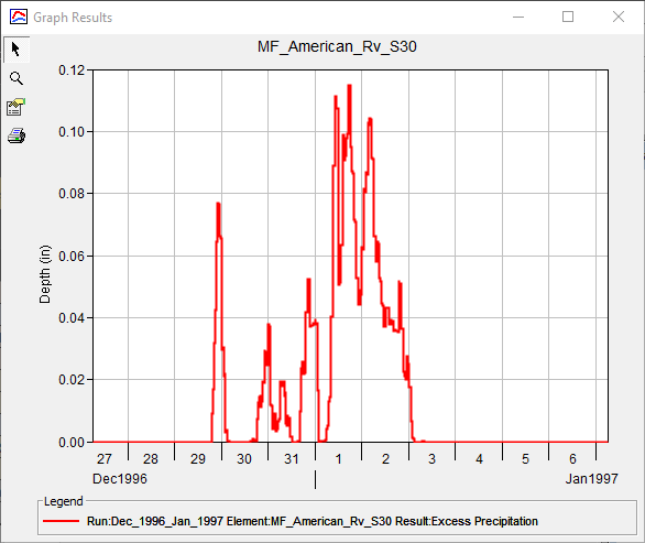
Question 1: What is the maximum excess precipitation rate (in inches/hour) that was realized within the Dec_1996_Jan_1997 simulation?
The maximum excess precipitation depth during this simulation was approximately 0.11 inches within 15 minutes. Thus, the maximum excess precipitation rate in inches/hour can be calculated as: 0.11 in / 15 minutes * 60 minutes / 1 hour = 0.44 inches/hour.
Question 2: What are the calibrated Tc and R values for the Dec_1996_Jan_1997 simulation?
Tc = 3.2 hours and R = 2.9 hours.
Simulate Hypothetical Event Using Clark Parameters
Next, apply the calibrated parameters achieved during the Dec_1996_Jan_1997 simulation to a hypothetical event.
- Open the Clark Basin Model.
- Select the Clark simulation run from the Compute toolbar.
- Press the Compute All Elements button to run the simulation.
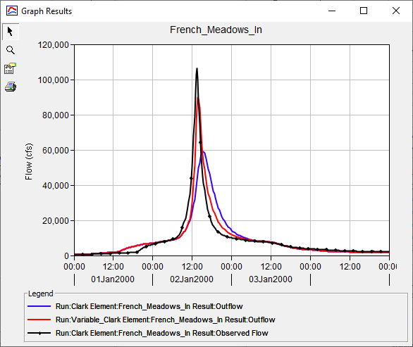
- Once the compute is complete, view the result graph and summary table for the French_Meadows_In junction element, as shown in the following figure. The computed results are shown in blue while the 2D Diffusion Wave results are shown in black.

Question 3. How do the Clark results compare against the 2D Diffusion Wave results?
The 2D Diffusion Wave results are much more piqued than the Clark results. Most notably, the Clark peak discharge of 59100 cfs is approximately half as large as the 2D Diffusion Wave peak discharge of 106800 cfs. Also, the Clark time of peak is occurs approximately 1.45 hours after the 2D Diffusion Wave time of peak. The runoff volumes are essentially the same.
Estimate Variable Clark Parameters
Regression equations that can be used to predict Variable Clark unit hydrograph parameters were developed for the state of California as part of Task 8 within the Memorandum of Agreement between HEC and DSOD. These equations relate physically measurable watershed characteristics (e.g. longest flow path) to ratios of Tc and R. Separate regression equations were developed for ratios of Tc and R to index parameters for all of the aforementioned excess precipitation rates. The same predictive variables were chosen for each excess precipitation rate to ease the use of the regression equations and mitigate the potential for sharp inflection points in the output or increasing ratios of Tc and R as excess precipitation rates increase for reasonable parameter values. A summary of the regression equations for each excess precipitation rate is presented within the following table.
| Excess Precipitation Rate (in/hr) | Equation | ||||
|---|---|---|---|---|---|
0.25 |
| ||||
0.5 |
| ||||
1.0 |
| ||||
2.0 |
| ||||
3.0 |
| ||||
4.0 |
| ||||
5.0 |
| ||||
6.0 |
|
where DA = drainage area (sq mi); S_{10-85} = average slope of the flowpath represented by 10 to 85 percent of the longest flow path (ft/ft); L_{c a} = centroidal longest flowpath length (mi); BR = basin relief (feet); and RR = relief ratio (dimensionless).
Designate Index Parameters
Question 4. Report the Excess Precipitationindex, Tcindex and Rindex values realized during the Dec_1996_Jan_1997 simulation.
Recall that the maximum excess precipitation rate was 0.44 inches/hour, the calibrated Tc was 3.2 hours, and the calibrated R was 2.9 hours. Thus, Excess Precipitationindex = 0.44 in/hr, Tcindex = 3.2 hr, and Rindex = 2.9 hr.
Extract Basin Characteristics and Estimate Ratios of Tcindex and Rindex
- Compute basin characteristics for the MF_American_Rv_S30 subbasin element by selecting Parameters | Characteristics | Subbasin, as shown within the following figure.

- HEC-HMS will populate characteristics for each subbasin element within the basin model, as shown within the following figure.

Next, use the regression equations presented above to estimate ratios of Tcindex and Rindex for excess precipitation rates of 0.25, 0.5, 1, 2, 3, 4, 5, and 6 in/hr, as shown below.
Predicted Tcindex Ratio for Excess Precip Rate (in/hr) Excess Precipitation Rate (in/hr) 0.25 0.5 1 2 3 4 5 6 Ratio 2.333119 1.454922 0.988565 0.708519 0.582986 0.532785 0.492662 0.45718 Predicted Rindex Ratio for Excess Precip Rate (in/hr) Excess Precipitation Rate (in/hr) 0.25 0.5 1 2 3 4 5 6 Ratio 5.624447 3.593561 1.659284 0.741164 0.512476 0.426392 0.353905 0.317881 Next, divide each of the aforementioned excess precipitation rates by the index excess precipitation rate of 0.44 in/hr and multiply by 100 to determine % Excess Precipitationindex. Also, multiply the Tcindex and Rindex ratios by 100 to determine % Tcindex and % Rindex. The resultant relationships are tabulated below.
% Excess Precipitationindex % Tcindex % Rindex 56.8 233.3 562.4 113.6 145.5 359.4 227.3 98.9 165.9 454.5 70.9 74.1 681.8 58.3 51.2 909.1 53.3 42.6 1136.4 49.3 35.4 1363.6 45.7 31.8 Next, add two additional points representing (0, Tcindex, Rindex) and (100, Tcindex, Rindex), as shown below.
% Excess Precipitationindex % Tcindex % Rindex 0 100 100 56.8 233.3 562.4 100 100 100 113.6 145.5 359.4 227.3 98.9 165.9 454.5 70.9 74.1 681.8 58.3 51.2 909.1 53.3 42.6 1136.4 49.3 35.4 1363.6 45.7 31.8 Finally, set ratios of Tcindex and Rindex greater than 100% to 100%. This ensures that no values greater than Tcindex and Rindex are used, as shown below.
% Excess Precipitationindex % Tcindex % Rindex 0 100 100 56.8 100 100 100 100 100 113.6 100 100 227.3 98.9 100 454.5 70.9 74.1 681.8 58.3 51.2 909.1 53.3 42.6 1136.4 49.3 35.4 1363.6 45.7 31.8 - The predicted and final relationships are plotted below.

- A close up of these relationships focusing on the values of interest are shown below.

Download a file containing the regression equations and basin characteristics here - MF_AmericanRv_Variable_Clark_Parameters.xlsx
Simulate Hypothetical Event Using Variable Clark Parameters
Now that you have defined the variable Tc and R relationships, input them as new shared data components within HEC-HMS and use them within the Variable Clark unit hydrograph method.
- Click Components | Paired Data Manager.
- Change the Data Type to Percentage Curves and click New.
- Name the new Percentage Curve MF_American_Rv_S30_Tc.
- Repeat the previous steps to create another Percentage Curve called MF_American_Rv_S30_R.
- Select the new Percentage Curves within the tree and enter the values for each, as shown in the following figure. For simplicity, non-essential ordinates were removed.

- Now, create a new Basin Model that can make use of these curves. Right click on the Clark Basin Model and select Create Copy...
- Name the new Basin Model Variable_Clark.
- Select the Variable_Clark Basin Model withn the Project Explorer tree.
- Select the MF_American_Rv_S30 subbasin element.
- Select the Transform tab.
- Change the Method to Variable Parameter, enter a Tc of 3.2 hr, an R of 2.9, an Index Excess of 0.44 in/hr, and select the two previously created Percentage Curves. The Variable Clark Component Editor should resemble the following figure.

- Select Compute | Create Compute | Simulation Run.
- Name the new simulation Variable_Clark.
- Select the Variable_Clark Basin Model, the Hypothetical Meteorologic Model, and the Hypothetical Control Specifications.
- Select the Hypothetical Meteorologic Model within the Project Explorer tree.
- Select the Basins tab.
- Toggle the drop down menu for the Variable_Clark Basin Model to Yes, as shown in the following figure.

- Select the Variable_Clark simulation run from the Compute toolbar.
- Press the Compute All Elements button to run the simulation.
- Once the compute is complete, view the result graph and summary table for the French_Meadows_In junction element, as shown in the following figure. The computed results are shown in blue while the 2D Diffusion Wave results are shown in black.

Question 5. How do the Variable Clark results compare against the 2D Diffusion Wave results at the French_Meadows_In junction element? How do the Variable Clark results compare against the Clark results?
The Variable Clark results more closely match the 2D Diffusion Wave results. The Variable Clark peak discharge of 89250 cfs is approximately 17550 cfs less than the 2D Diffusion Wave peak discharge of 106800 cfs. Also, the Variable Clark time of peak occurs at nearly the same time as the 2D Diffusion Wave time of peak. A summary of the Clark, Variable Clark, and 2D Diffusion Wave results at the French_Meadows_In junction element are shown below.
| Statistic | Clark | Variable Clark | 2D Diffusion Wave |
|---|---|---|---|
| Peak Discharge (cfs) | 59125 | 89250 | 106800 |
| Time of Peak Discharge | 1/2/2000 15:15 | 1/2/2000 13:45 | 1/2/2000 13:30 |
| Volume (in) | 28.01 | 28.01 | 27.54 |
A plot of these results are shown in the following figure. The Clark results are shown in blue, the Variable Clark results are shown in red, and the the 2D Diffusion Wave results are shown in black.
Question 6. For the period ending 02Jan2000 12:15?, what was the excess precipitation rate (in inches/hr)? What percentage of the Excess Precipitationindex does this represent? For the same time period, what Tc and R were used? What percentage of the Tcindex and Rindex does this represent?
Using the output from the Results tab | Simulation Runs | Variable_Clark | MF_American_Rv_S30 | Excess Precipitation time series, the excess precipitation for the 15-min time step ending at 02Jan2000 12:15 was 1.0 inches. Thus, the excess precipitation rate in inches/hour can be calculated as: 1.0 in / 15 minutes * 60 minutes / 1 hour = 4.0 inches/hour. This represents 909% of the index excess precipitation rate (i.e. 4 in/hr / 0.44 in/hr).
From the console output, the Tc and R for the period ending 02Jan2000 12:15 were 1.71 hr and 1.24 hr, respectively, as shown in the following image. This represents 53.3% and 42.6% of Tcindex and Rindex, respectively.

The excess precipitation, Tc, and R values that were realized or used for each time step are shown in the figure below.
