Download PDF
Download page Discharge-Frequency Curve Development Using HEC-SSP.
Discharge-Frequency Curve Development Using HEC-SSP
Last Modified: 2023-02-16 20:31:20.824
This tutorial demonstrates a process to estimate a flow-frequency curve using observed data and Bulletin 17C procedures.
Software Version
HEC-SSP version 2.3 was used to develop this tutorial.Project Files
Download the initial project files here:
Introduction
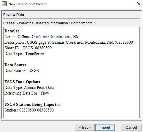
The purpose of this step is to develop a discharge-frequency curve for the USGS gage at Gallinas Creek near Montezuma, NM (USGS Station ID 08380500) using HEC-SSP (version 2.3). This discharge-frequency curve will be used to calibrate (inform parameter value adjustments) for the Gallinas Creek Watershed HEC-HMS model. This example illustrates the computation of a peak flow frequency curve using Expected Moments Algorithm (EMA) and Bulletin 17C procedures (England et al. 2019) with an annual maximum series comprised of a broken record of systematic flood peaks.
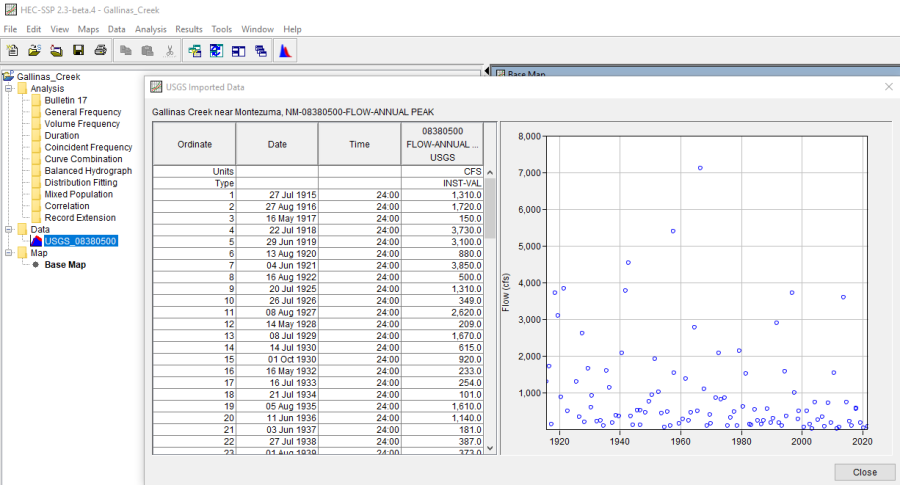
The Gallinas Creek near Montezuma, NM (USGS gage location) has a drainage area of 84 square miles. The USGS Gage 08380500 has an annual peak record consisting of 107 peaks beginning in 1915 and ending in 2021. There is one "broken record" period where the gage was discontinued: 1923-1924. Thus, there are two years of missing data at this gage during the period of record. There were no historic flood records located for this gage. The USGS operated a streamgage (Gallinas Creek at Montezuma, NM, USGS Station ID 08381000) located slightly downstream of USGS gage 08380500 from 1904 to 1966. The Gallinas Creek at Montezuma, NM (USGS gage location) has a drainage area of 87 square miles. Information from USGS 08381000 can be used to inform the perception threshold to represent the two years of missing information.
Using the HEC-SSP Data Import Wizard
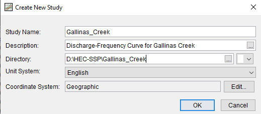
- Open HEC-SSP and Create a New Study for Gallinas Creek.
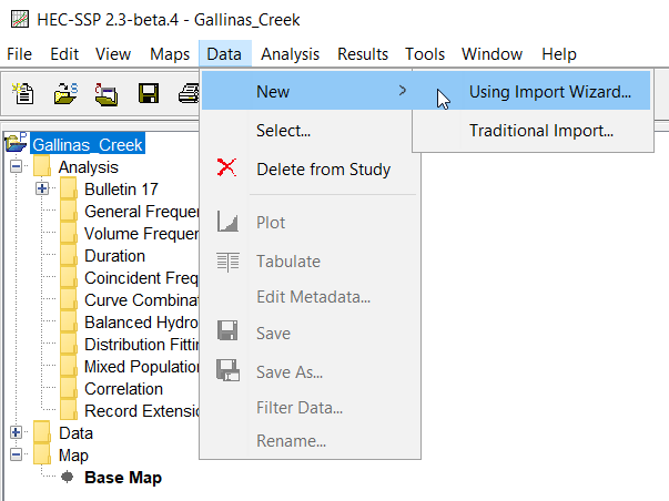
- Use the data import wizard to import the annual peak flow data for the USGS gage at Gallinas Creek near Montezuma, NM (USGS Station ID 08380500) (Data | New | Using Import Wizard…).
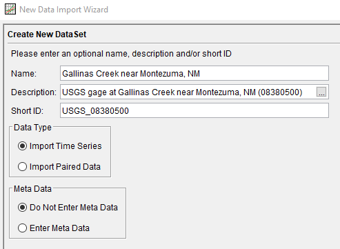
- Enter a name, description, and short ID for the new data set.
- Select Import Time Series as the data type.
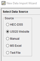
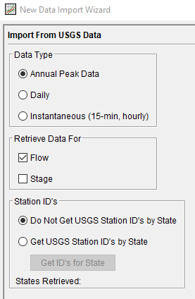
- Select USGS Website as the source.
- Select Annual Peak Data as the data type.
- Check the box next to Retrieve Data for Flow.
- Select Do Not Get USGS Station ID's by State because the USGS station ID is already known.
- Check the Import Data box for the first row of the first column in the table.
- Enter the USGS station ID in the first row of the second column in the table.
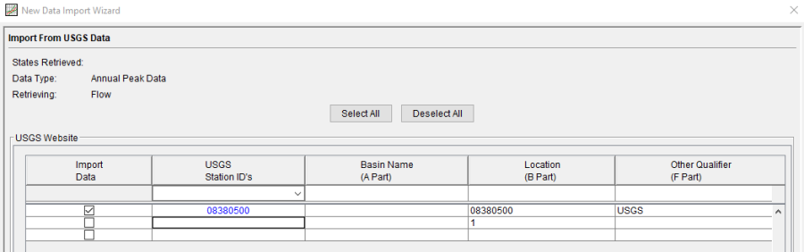
- Review the data and click Import.
- Imported data will be located under the Data folder in the study directory. The data is saved to the project's DSS file. The data can be visualized by right clicking on the DSS file containing the imported data and selecting Plot or Tabulate.
- Note: Due to the limited time to complete the initial Gallinas Creek analysis, the imported dataset was assumed to be independent and identically distributed (IID). This is a high elevation watershed that has the potential to have three different meteorological storm events: snow-melt runoff, rain on snow runoff, and rainfall runoff. Time permitting, the separation of the datasets into their various mechanisms may help with calibration of the hydrologic and hydraulic models. There are tools within HEC-SSP that can be used to help filter and modify the datasets. See Filter and Modify Several Data Sets.
Creating a Bulletin 17C Analysis
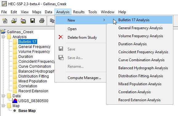
- Create a new Bulletin 17C analysis (Analysis | New | Bulletin 17 Analysis).
- Enter a name and description. Select the flow data set that was imported during the previous step.
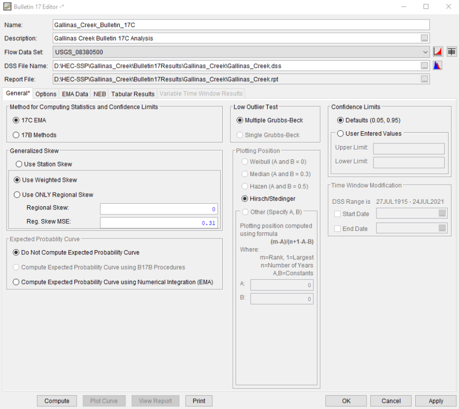
- Under the General tab, select the desired method for computing statistics and confidence limits.
- In this case, 17C EMA was selected to perform a Bulletin 17C analysis using the Expected Moments Algorithm.
- Select the desired method for generalized skew.
- In this case, Use Weighted Skew was selected.
- The regional skew was set to 0 and the regional skew mean squared error (MSE) was set to 0.31. These values were based on a study analyzing the magnitude and frequency of peak discharge and are specific to New Mexico (Waltemeyer, 2008). Studies and equations from other regions, specific to the project area, should be used to determine the appropriate skew values to use.
- Select the desired confidence limits.
- In this case, the Defaults (0.05, 0.95) were selected.
- In this case, the Defaults (0.05, 0.95) were selected.
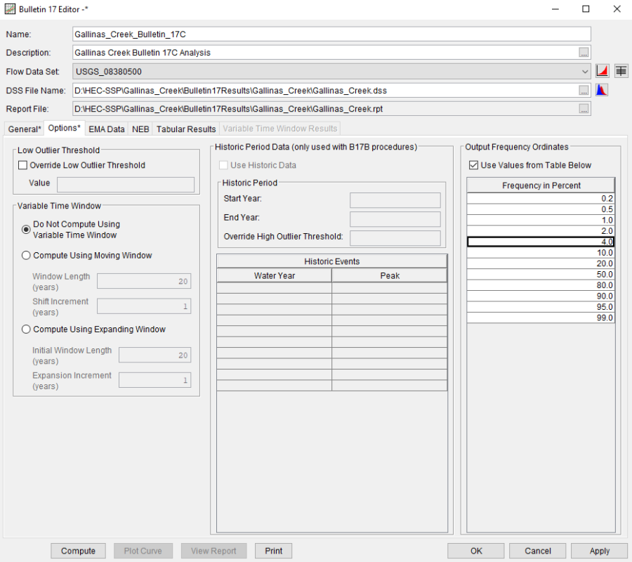
- Under the Options tab, select Do Not Compute Using Variable Time Window for the variable time window options.
- Check the box to Use Values from the Table Below under the Output Frequency Ordinates section. Change the frequency in percent from 5.0 to 4.0 to obtain results for an annual exceedance probability of 4% (25-year return period) instead of an annual exceedance probability of 5% (20-year return period).
- This step is needed so that the HEC-SSP and HEC-HMS results can be directly compared because the NOAA Atlas 14 data used in the HEC-HMS model is only provided for a 25-year return period, not a 20-year return period.
- This step is needed so that the HEC-SSP and HEC-HMS results can be directly compared because the NOAA Atlas 14 data used in the HEC-HMS model is only provided for a 25-year return period, not a 20-year return period.
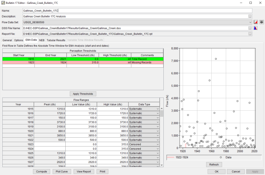
- Under the EMA Data tab, add the missing data to the perception thresholds table. 17C EMA requires a non-zero-to-infinite perception threshold for all periods of missing data. Use historical information if it is available to inform perception thresholds for periods of missing data.
- Identify years with missing data (1923 and 1924). For this analysis, only one perception thresholds is required because there is only one period of time with missing data.
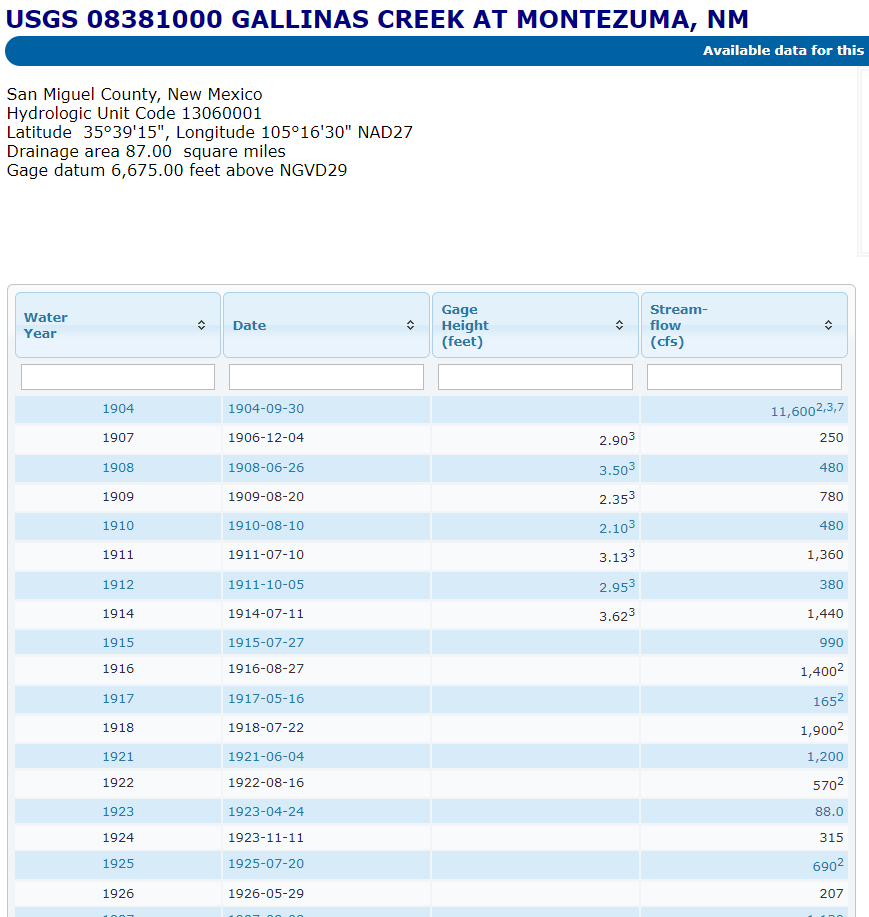
- In this case, a USGS streamgage (Gallinas Creek at Montezuma, NM, USGS Station ID 08381000) no longer in operation, located slightly downstream of USGS 08380500 can be used to inform the perception thresholds for the period of missing annual-peak flow data. According to annual-peak flow records at USGS 08381000, the annual-peak flow rates for 1923 and 1924 were 88 and 315 cfs, respectively. Therefore, 315 cfs can be used as the low threshold which implies that had a flood event occurred with an annual-peak flow greater than 315 cfs it would have been documented or USGS 08381000 would have recorded a larger value.
- In the Perception Thresholds table, enter 1923 as the start year and enter 1924 as the end year.
- Enter 315 as the low threshold.
- Set the high threshold to Infinity (INF) by double clicking on the cell to edit, then right clicking and selecting Set as INF.
- Add a description (Missing Records) to the comments column.
- Click Apply Thresholds.
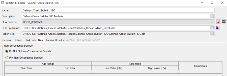
- Under the NEB tab, select Do Not Plot Non-Exceedance Bounds for the non-exceedance bounds options.
- Compute the discharge-frequency curve by clicking Compute.
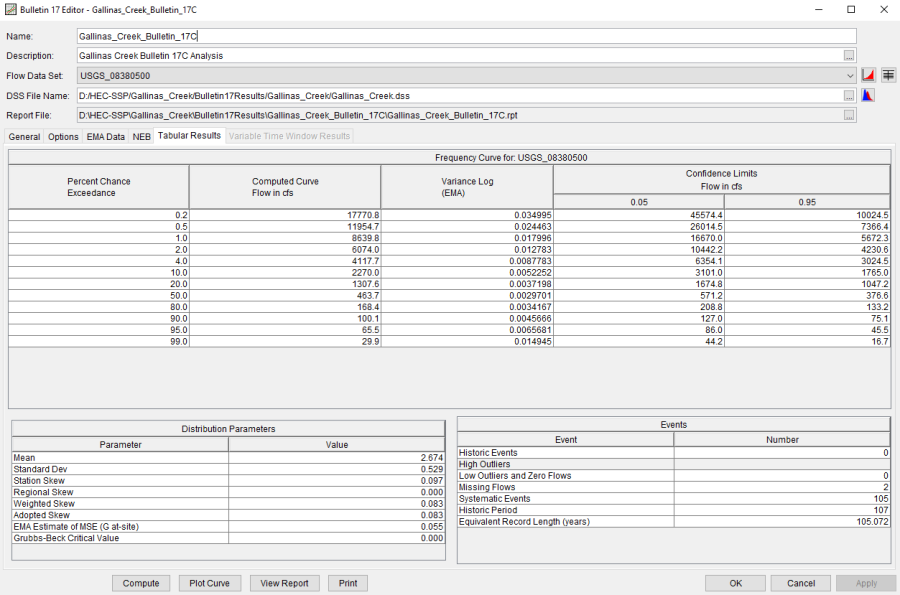
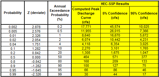
- Under the Tabular Results tab, the computed curve, confidence limits, and distribution parameters can be viewed.
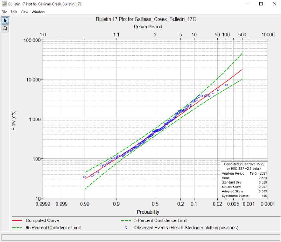
- Click Plot Curve to view the computed curve.
- Under the Tabular Results tab, the computed curve, confidence limits, and distribution parameters can be viewed.
Plotting Results
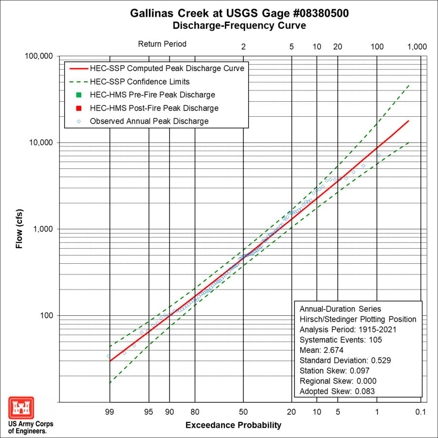
- Copy the computed results into the Discharge_Frequency_Curve_Gallinas_Creek_Watershed spreadsheet to plot the discharge-frequency curve to compare to the HEC-HMS results. In a following workshop, the loss and transform parameters in the pre-fire HEC-HMS model will be adjusted to generate results that are comparable to the discharge-frequency curve computed following Bulletin 17C procedures. Copy the computed curve and confidence limits flow values for each percent chance exceedance and paste the values into the spreadsheet.
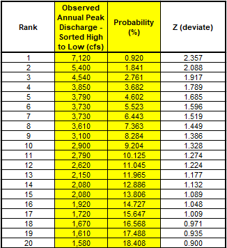
- Copy the observed annual peak discharge values and their corresponding plotting positions from the curve plot.
- When an HEC-SSP Frequency Curve plot is open, click File | Tabulate to view the data points in the plot.
- Double click on the Flow heading for the Observed Events column to sort the annual peak flow values from high to low.
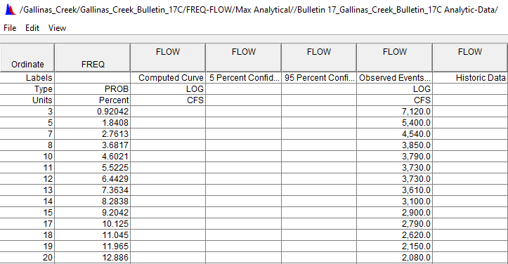
- Copy the annual peak flow values and corresponding probability values into the spreadsheet.
- Record the 17C analysis parameters in the discharge-frequency curve plot.
References
England, J.F. Jr., Cohn, T. A., Faber, B. A., Stedinger, J. R., Thomas, W. O., Veilleux, A. G., Kiang, J. E., and Robert R. Mason Jr. 2019. "Guidelines for Determining Flood Flow Frequency Bulletin 17C, Chapter 5 of Section B, Surface Water." Book 4, Hydrologic Analysis and Interpretation, Techniques and Methods 4-B5, Version 1.1, U.S. Geological Survey, Reston, VA.
Waltemeyer, S.D., 2008, Analysis of the magnitude and frequency of peak discharge and maximum observed peak discharge in New Mexico and surrounding areas: U.S. Geological Survey Scientific Investigations Report 2008–5119, 105 p.
Project Files
