Download PDF
Download page Gradation Curve Development Procedure.
Gradation Curve Development Procedure
Last Modified: 2023-03-24 16:06:36.249
This tutorial demonstrates procedures to develop gradation curves for HEC-HMS modeling.
Software Version
ArcPro and HEC-HMS 4.11 were used to create this example.Project Files
Download the initial project files here:
Download a copy of the gSSURGO database for New Mexico at: https://drive.hecdev.net/share/G8TtpHSx

Introduction
When using the erosion and sediment transport components in HEC-HMS, a gradation curve is a required input for some of the specific methods. For the surface erosion methods, the bulk sediment discharge, which includes all grain sizes, is computed for each subbasin element. A gradation curve, defined by the user for each subbasin, specifies the proportion of the total sediment discharge that should be apportioned to each grain size class or subclass. A different gradation curve can be used at each subbasin to represent differences in the downstream erosion, deposition, and resuspension processes.
All of the sediment transport methods for reach elements require the input of an initial gradation curve to define the distribution of the bed sediment by grain size class at the beginning of the simulation. This can change during the simulation depending upon erosion and deposition from specific grain size classes. Finally, for reservoir elements using the specified sediment method, a gradation curve is used to apportion the total sediment discharge from the reservoir into grain size classes.
The purpose of this procedure is to present three options for developing gradation curves depending on the timeframe, application, and level of detail needed for a given watershed assessment:
- Placeholder data
- Use with subbasin elements only.
- Use when total sediment load is needed and sediment load by grain class is not needed.
- Total sediment load results can be used to compute a bulking factor/volumetric sediment concentration for each subbasin or for the entire watershed.
- Appropriate for use in emergency applications or situations with limited time, funding, and soil data available.
- gSSURGO data
- Use with subbasin, reach, or reservoir elements.
- Use when sediment load by grain class is needed for subbasin elements.
- Use when sediment methods for reaches or reservoir elements require the input of a gradation curve. Note that while this database relies on physical samples collected by the U.S. Department of Agriculture, Natural Resources Conservation Service (USDA-NRCS), rarely is the sampling performed in reach locations, so the extracted grain class may be finer than actually exists within an environment subject to fluvial sorting.
- Appropriate for use in situations when physical samples are not available or cannot be collected within the timeframe or funding available.
- Physical soil sample data
- Use with subbasin, reach, or reservoir elements.
- Use when sediment load by grain class is needed for subbasin elements.
- Use when sediment methods for reaches or reservoir elements require the input of a gradation curve.
- Use when physical samples are already available or when the timeframe and funding permit the collection of physical samples.
Selecting a Grade Scale
It should be noted that the gradation scale option needs to be considered once the gradation curve range is known. The results for the sediment load/volume are calculated independently of the gradation curve, however, the chosen gradation scale may limit the reported sediment load/volume for that subbasin, as illustrated in the following table.
Grade Scale | ||
Gradation Curve Range | Clay Silt Sand Gravel (0.002 mm – 64 mm) | AGU 20 (0.002 mm – 2048 mm) |
Clay (0.002mm) to Gravel (64 mm) | Covers all grain classes – no sediment load/volume limitations | Covers all grain classes – no sediment load/volume limitations |
Clay (0.002mm) to Large Boulder (2048 mm) | Underestimates sediment load/volume (excludes volume associated with all grain classes > 64mm) – reported sediment load/volume is reduced by the percent of the grain sizes larger 64 mm | Covers all grain classes – no sediment load/volume limitations |
Developing a Gradation Curve with Placeholder Data
In this option, a single gradation curve is developed using placeholder data to allow the HEC-HMS model to run for the surface erosion methods. It should be noted that this gradation curve does not affect the computation of the bulk sediment discharge for each subbasin element. Only the total sediment load results should be utilized with this option. The results for the sediment load by grain class computed using the placeholder data are not representative of the specific watershed being modeled and should not be used.
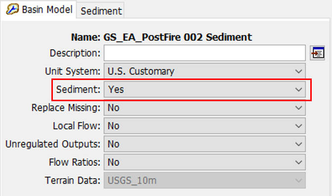
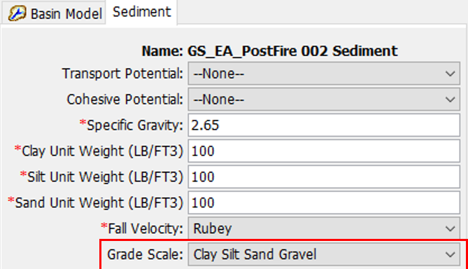
- Select the appropriate Grade Scale to be used with each basin model in HEC-HMS.
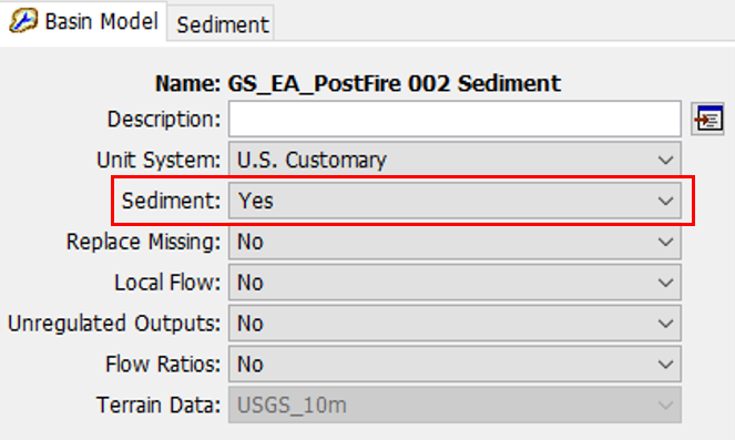
- When sediment simulations are toggled on (selection of Yes under the Sediment tab when the basin is selected) there will be two types of grade scale that can be selected under the Sediment tab: Clay Silt Sand Gravel or AGU 20. The selected grade scale controls how many grain size classes are utilized in the sediment simulations.
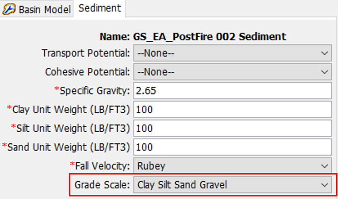
- The Clay Silt Sand Gravel grade scale will take the entered gradations and lump them into clay (0.002 to 0.004 mm), silt (0.004 to 0.0625 mm), sand (0.0625 to 2 mm), and gravel (2 to 64 mm) size classes. If an entered gradation has material greater than 64 mm, this will not be taken into consideration during the sediment simulation. Note as stated above in Selecting a Grade Scale, this will underestimate the sediment yield for this subbasin. This may be a reasonable assumption if the subbasin results will be compiled at a downstream station where the larger sediment sizes are not expected to be transported.
- If a greater level of detail is desired, the AGU 20 grade scale can be selected which splits the entered gradation into 20 categories ranging from large boulders (2048 mm) to clay. Only the boulder, cobble, gravel, sand, and silt size classes have finer gradations. The clay size class in the AGU 20 grade scale is still lumped together like the Clay Silt Sand Gravel grade scale.
- In this case, the Clay Silt Sand Gravel grade scale was used.
- When sediment simulations are toggled on (selection of Yes under the Sediment tab when the basin is selected) there will be two types of grade scale that can be selected under the Sediment tab: Clay Silt Sand Gravel or AGU 20. The selected grade scale controls how many grain size classes are utilized in the sediment simulations.
- Enter gradation curve data as paired data in HEC-HMS.
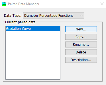
- Select Components | Paired Data Manager.
- For data type, select Diameter-Percentage Functions.
- Click New to create a paired data.
- Type a name and description for function and click Create.
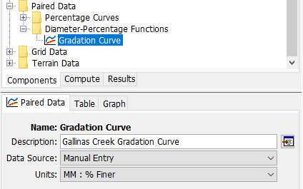
- Once the gradation curve is created, define the data source and units.
- For data source, select Manual Entry.
- For units, select MM: % Finer. Note: This is chosen since gradation curves tend to be defined (and thus more readily available) in terms of millimeters instead of inches.
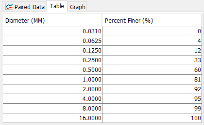
- Manually enter the gradation curve data.
- Select the Table tab.
- Enter the soil diameters from largest to smallest or smallest to largest.
- Enter the corresponding percent finer for each soil diameter.
The following values can be entered as placeholder data for the gradation curve:
Diameter (mm) Percent Finer (%) 0.031
0
0.0625
4
0.125
12
0.25
33
0.5
60
1
81
2
92
4
95
8
99
16
100
Developing a Gradation Curve with gSSURGO Data
In this option, a single gradation curve representative of the Gallinas Creek Watershed soil conditions is developed using data from the Gridded Soil Survey Geographic (gSSURGO) database from the USDA-NRCS. ESRI ArcGIS Pro (version 3.0.2) and Microsoft Excel are used to complete this analysis. It should be noted that this gradation curve does not affect the computation of the bulk sediment discharge for each subbasin element. It is used to specify the proportion of the total sediment discharge to each grain size class, shown in the sediment load by grain class results. In this procedure, the gSSURGO data is sampled for the entire watershed to represent the subbasin elements. To apply this procedure to reach and reservoir elements, the gSSURGO data specific to those elements, rather than the entire watershed, should be sampled. However, the gSSURGO database is usually missing data for fluvial channels which may necessitate the collection of physical samples or other soil data.
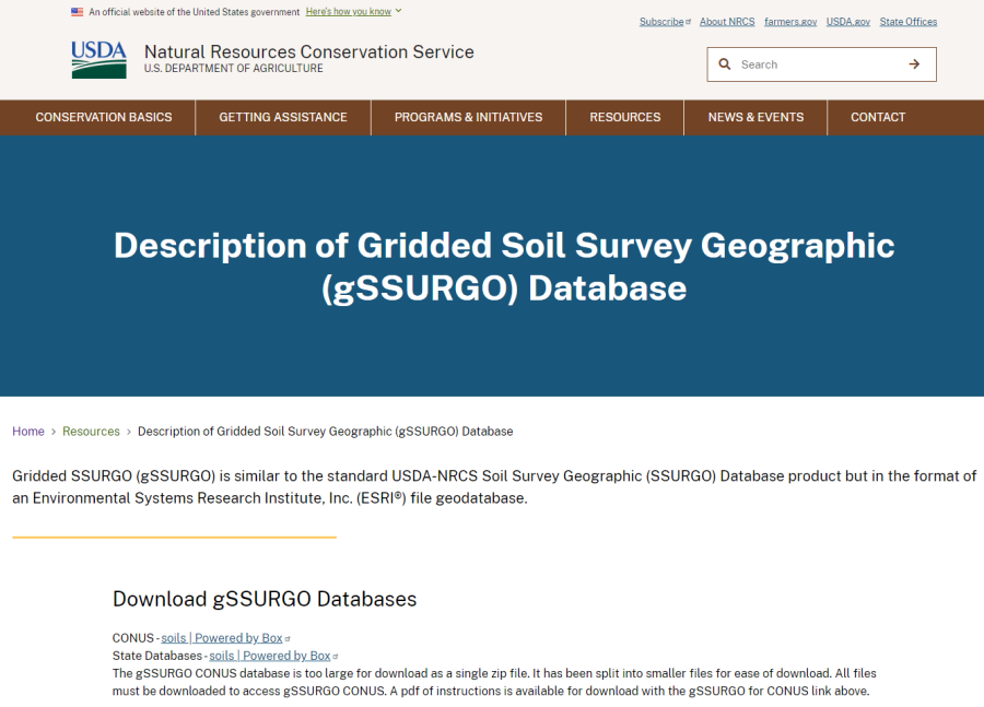
- Download the gSSURGO database from the USDA-NRCS website for the project area.
- Navigate to the USDA-NRCS gSSURGO database website: https://www.nrcs.usda.gov/resources/data-and-reports/description-of-gridded-soil-survey-geographic-gssurgo-database.
- Click on the State Databases - Soils link to download the gSSURGO database by state: https://nrcs.app.box.com/v/soils/folder/180112652169.
- Select the appropriate state database and download the .zip file.
- In this case, the New Mexico (NM) state database was downloaded.
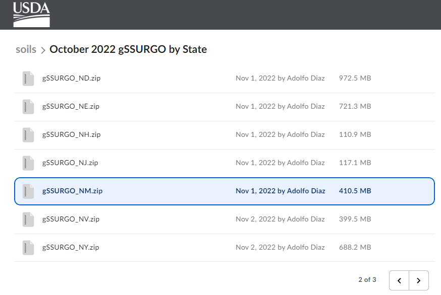
- In this case, the New Mexico (NM) state database was downloaded.
- Unzip the downloaded folder to extract the gSSURGO geodatabase file (.gdb).
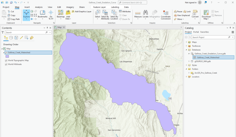
- Open ArcGIS Pro and Create a New Project for the Gallinas Creek gradation curve.
- Add a shapefile (.shp) of the project area to the map. The gradation curve will be defined based on the soil data contained within this area.
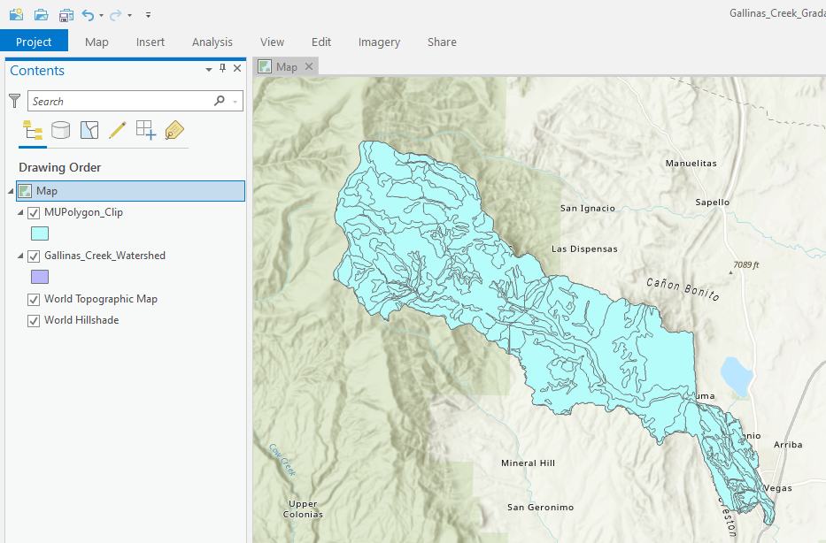
- In this case, the project area is defined by the extents of the Gallinas Creek Watershed delineated in HEC-HMS.
- Add the Gallinas_Creek_Watershed shapefile, located in the Gallinas_Creek_Gradation_Curve geodatabase, to the map.
- Add the gSSURGO database file to the project catalog and clip the dataset to the project area.
- Add the Map Unit Polygon (MUPOLYGON) layer to the map. Either click Add Data and select the file or use the Catalog pane, select the file, and drag and drop into the map environment.
- Use the Clip analysis tool (Analysis Tools | Extract | Clip) to trim the MUPOLYGON layer to the project area.
- Select MUPOLYGON as the input features.
- Select Gallinas_Creek_Watershed shapefile as the clip features.
- Type a name for the output features.
- Click Run.

- Identify the tables and column groups from the gSSURGO database that contain soil data of interest.
- A full description of each of the tables in the gSSURGO database is provided here: https://www.nrcs.usda.gov/sites/default/files/2022-08/SSURGO-Metadata-Table-Column-Descriptions-Report.pdf
- The Horizon (CHORIZON) table contains the following column groups that are utilized in the gradation curve development:
- Rock > 10 – percent by weight of the horizon occupied by rock fragments greater than 10 inches in size.
- Rock 3-10 – percent by weight of the horizon occupied by rock fragments 3-10 inches in size.
- #4 – soil fraction passing a #4 sieve (4.70 mm opening) as a weight percentage of the less than 3 inch (76.4 mm) fraction.
- #10 – soil fraction passing a #10 sieve (2.0 mm opening) as a weight percentage of the less than 3 inch (76.4 mm) fraction.
- #40 – soil fraction passing a #40 sieve (0.42 mm opening) as a weight percentage of the less than 3 inch (76.4 mm) fraction.
- #200 – soil fraction passing a #200 sieve (0.074 mm opening) as a weight percentage of the less than 3 inch (76.4 mm) fraction.
- Total Sand – mineral particles 0.05 mm to 2.0 mm in equivalent diameter as a weight percentage of the less than 2.0 mm fraction.
- Very Coarse Sand (vcos) – mineral particles 1.0 mm to 2.0 mm in equivalent diameter as a weight percentage of the less than 2.0 mm fraction.
- Coarse Sand (cos) – mineral particles 0.5 mm to 1.0 mm in equivalent diameter as a weight percentage of the less than 2.0 mm fraction.
- Medium Sand (ms) – mineral particles 0.25 mm to 0.5 mm in equivalent diameter as a weight percentage of the less than 2.0 mm fraction.
- Fine Sand (fs) – mineral particles 0.10 mm to 0.25 mm in equivalent diameter as a weight percentage of the less than 2.0 mm fraction.
- Very Fine Sand (vfs) – mineral particles 0.05 mm to 0.10 mm in equivalent diameter as a weight percentage of the less than 2.0 mm fraction.
- Total Silt – mineral particles 0.002 mm to 0.05 mm in equivalent diameter as a weight percentage of the less than 2.0 mm fraction.
- Coarse Silt – mineral particles 0.02 mm to 0.05 mm in equivalent diameter as a weight percentage of the less than 2.0 mm fraction.
- Fine Silt – mineral particles 0.002 mm to 0.02 mm in equivalent diameter as a weight percentage of the less than 2.0 mm fraction.
- Total Clay – mineral particles less than 0.002 mm in equivalent diameter as a weight percentage of the less than 2.0 mm fraction.
- The Representative Value (RV) for each category will be used for the gradation curve development.
- Join the identified table(s) to the MUPolygon_Clip layer using attribute columns that are common between tables.
- The data of interest is contained in the CHORIZON table which is organized by Component Key (COKEY). The data in the MUPolygon_Clip layer is organized by Map Unit Key (MUKEY). The Component table contains both the COKEY and MUKEY attributes and can be used to join data from the CHORIZON table to the MUPOLYGON_Clip layer. Both the CHORIZON and the Component tables must be added to the map. This can be done by selecting them in the Catalog pane then dragging and dropping them in the Contents pane. They will show up as standalone tables.
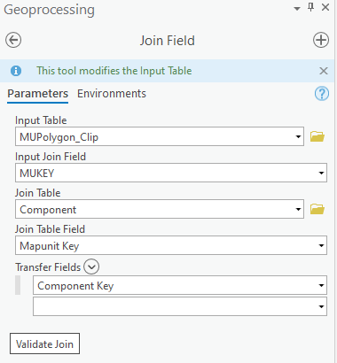
- Use the Join Field data management tool (Data Management Tools | Joins | Join Field) to join the COKEY attribute column from the Component table to the MUPolygon_Clip layer.
- Select MUPolygon_Clip as the input table.
- Select MUKEY as the input join field.
- Select Component as the join table.
- Select Mapunit Key as the join table field.
- Select Component Key as the transfer fields.
- Click Run. You should see the COKEY field added to the MUPolygon_Clip attribute table.
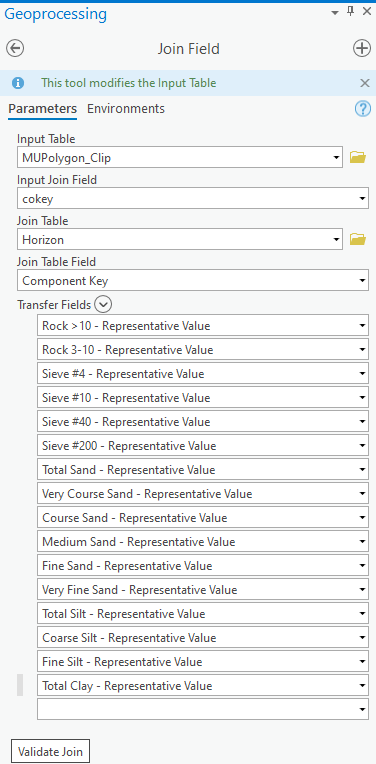
- With the first join completed, use the Join Field data management tool (Data Management Tools | Joins | Join Field) to join the data of interest from the CHORIZON table to the MUPolygon_Clip layer.
- Select MUPolygon_Clip as the input table.
- Select Component Key as the input join field.
- Select Horizon as the join table.
- Select Component Key as the join table field.
- Select all of the column groups identified in Step 5 as the transfer fields.
- Click Run.
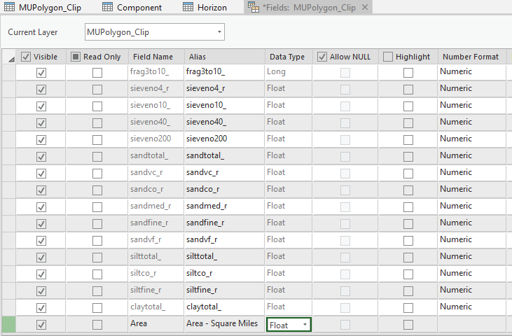
- Calculate the area for each shape within the MUPolygon_Clip layer.
- Open the attribute table and click Add Field.
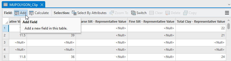
- Specify a Field Name, Alias, Data Type, and Number Format for the new field.
- Click Save in the ribbon at the top of ArcGIS Pro (the Fields ribbon). Then, the add field box can be closed. The Area - Square Miles field will show up in the MUPolygon_Clip attribute table.
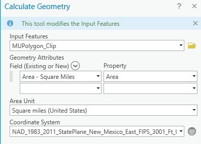
- In the MUPolygon_Clip attribute table, right click on the new attribute column and select Calculate Geometry. Note: Ensure that only the column is selected. If a specific polygon was selected and then the column is selected, the calculation will only occur for the selected element and not for the entire feature.
- Select MUPolygon_Clip as the input features.
- Select the new attribute column as the geometry attributes.
- Select Area as the property.
- Select Square miles as the area unit.
- Select the appropriate coordinate system.
- Click Ok.
- Open the attribute table and click Add Field.
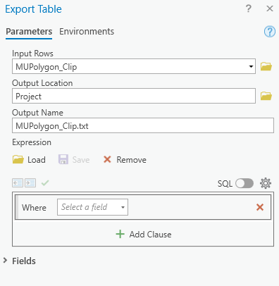
- Export the attribute table for the MUPolygon_Clip layer.
- Right click on the MUPolygon_Clip layer, click on Data, and click Export Table.
- Select MUPolygon_Clip as the input table.
- Specify a Output Location and Output Name for the output table.
- Click Ok. A new file will be created, you can open this file in Excel.
- Process the gSSURGO soil data in Excel to develop a gradation curve.
- Use the Gallinas_Creek_Gradation_Curve spreadsheet as a template. This spreadsheet is located at the beginning of this example.
- On the gSSURGO Data sheet:
- Copy and paste the exported data from the MUPolygon_Clip file into the appropriate columns in the spreadsheet.
- In this case, the data for each soil category is presented in percent by weight. Calculate the weighted area for each soil category by multiplying the percent by weight * area for each row.
- The sieve categories (#4, #10, #40, and #200) provide the percent passing the sieve opening as a percent of the sample volume less than 3 inches. Therefore, these percentages must be adjusted to reflect the entire sample volume. The correction is calculated as (100 minus the percent in the Rock > 10 category minus the percent in the Rock 3-10 category). This correction (expressed as a fraction) is multiplied by the weighted area.
- Sort the data so that the rows containing soil data are listed before the rows that are missing soil data. Sort the data using the Total Clay column, see below. This will make the calculations in the next step simpler.
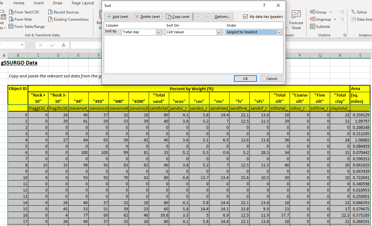
Rows 166 through 224 should have 0 defined for all categories.
- On the Gradation Curve sheet:
- Calculate the total area of the watershed with and without soil data available (Cell D30 and D31, respectively).
- Calculate the weighted area for each soil category.
- Sum the weighted area for each soil category computed on the gSSURGO Data sheet in Column F on the Gradation Curve sheet.
- The sieve categories are expressed as the percent finer area, and it is necessary to show the #4 Sieve as a percent within the 4.7 to 76.4 mm grain size class area. To compute the area containing rock between 4.7-76.4 mm in diameter, subtract the area for the Rock > 10, Rock 3-10, and #4 Sieve categories from the total area with data available (Cell F8).
- The other sieve categories can be corrected relative to one another using the #4 Sieve correction. For example, to compute the area containing rock between 2-4.7 mm in diameter, subtract the area for the #10 Sieve category from the area for the #4 Sieve category (Cell F10).
- For the sand, silt, and clay soil categories, the weighted area data corresponds to the percent of the total watershed area based on an assessment of the 2 mm fraction and finer soil volume. In order to relate this to the entire soil volume, the data needs to be apportioned to the area containing the soil fraction less than 2 mm in diameter indicated by the area calculated for the #10 Sieve category (soil fraction less than 2 mm in diameter) (Cell F11).
- In this case, 61.1 square miles of the Gallinas Creek Watershed contains soil data. 36.3 square miles (out of the 61.1 square miles) contain the soil fraction less than 2 mm in diameter. Therefore, the data for the sand, silt, and clay categories are apportioned to the area of 36.3 square miles (Column G).
- Calculate the percent by weight for each soil category by dividing the area for each soil category by the total area with data available (Column H).
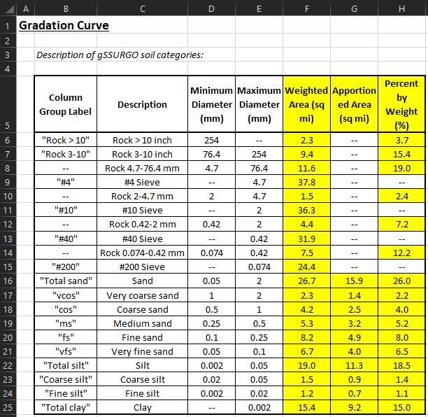
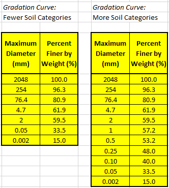
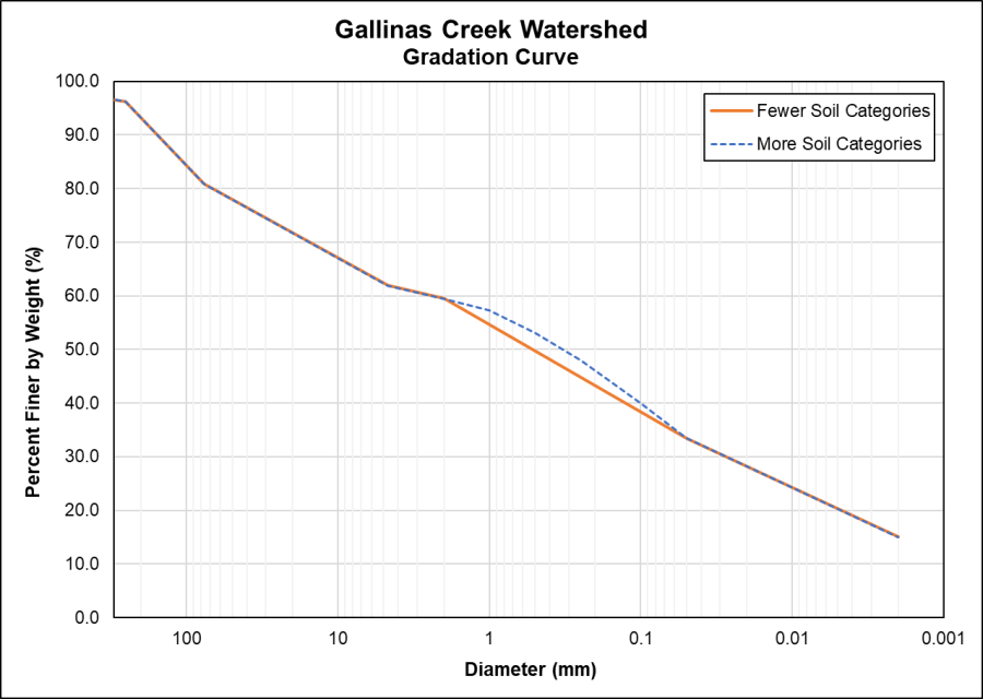
- Determine which soil categories to include in the gradation curve. In this case, two options are presented (fewer and more soil categories):
- In one option, the Total Sand category is used to define the sand portion (0.05-2 mm in diameter) of the gradation curve.
- In another option, the Very Coarse Sand, Coarse Sand, Medium Sand, Fine Sand, and Very Fine Sand categories are used to define the sand portion (0.05-2 mm in diameter) of the gradation curve.
- It should be noted that the Coarse Silt and Fine Silt categories were not used in either option for the gradation curve. These datasets were not complete, as indicated by the area for these categories not adding to the area for the Total Silt category. Therefore, the Total Silt category was used instead.
- The maximum diameter was set to 2048 mm based on the maximum diameter for boulders according to the AGU 20 grade scale.
- Calculate the percent finer by weight for each diameter. Starting with the smallest diameter, set the percent finer by weight equal to the percent by weight calculated for that soil category. For the next diameter, add the percent finer from the previous diameter to the percent by weight calculated for that soil category. Continue until the percent finer by weight is calculated for each diameter. The last value calculated should equal 100%.
- Entering a Gradation Curve into HEC-HMS:
- Select the appropriate Grade Scale to be used within each basin model in HEC-HMS.
- When sediment simulations are toggled on (select Yes under the Sediment tab when the basin is selected), there will be two types of grade scales that can be selected under the Sediment tab: Clay Silt Sand Gravel or AGU 20. The selected grade scale controls how many grain size classes are utilized in the sediment simulations.
- The Clay Silt Sand Gravel grade scale will take the entered gradations and lump them into clay (0.002 to 0.004 mm), silt (0.004 to 0.0625 mm), sand (0.0625 to 2 mm), and gravel (2 to 64 mm) size classes. If an entered gradation has material greater than 64 mm, this will not be taken into consideration during the sediment simulation. Note as stated above in Selecting a Grade Scale this will underestimate the sediment yield for this subbasin. This may be a reasonable assumption if the subbasin results will be compiled at a downstream station where the larger sediment sizes are not expected to be transported.
- If a greater level of detail is desired, the AGU 20 grade scale can be selected which splits the entered gradation into 20 categories ranging from large boulders (2048 mm) to clay. Only the boulder, cobble, gravel, sand, and silt size classes have finer gradations. The clay size class in the AGU 20 grade scale is still lumped together like the Clay Silt Sand Gravel grade scale.
- In this case, the Clay Silt Sand Gravel grade scale was used. (Note: For this simulation where it was desirable to calculate the debris yield at the watershed outlet without reach transport simulation, it was assumed that larger size classes (> 64 mm) would be deposited sufficiently upstream of the watershed outlet. Thus utilization of the Clay Silt Sand Gravel grade scale option, which reduces the debris volume based on the percent > 64 mm, was assumed to be reasonable.
- When sediment simulations are toggled on (select Yes under the Sediment tab when the basin is selected), there will be two types of grade scales that can be selected under the Sediment tab: Clay Silt Sand Gravel or AGU 20. The selected grade scale controls how many grain size classes are utilized in the sediment simulations.
- Enter gradation curve data as paired data in HEC-HMS.
- Select Components | Paired Data Manager.
- For data type, select Diameter-Percentage Functions.
- Click New to create a paired data.
- Type a name and description for function and click Create.
- Once the gradation curve is created, define the data source and units.
- For data source, select Manual Entry.
- For units, select MM: % Finer. Note: This is chosen since gradation curves tend to be defined (and thus more readily available) in terms of millimeters instead of inches.
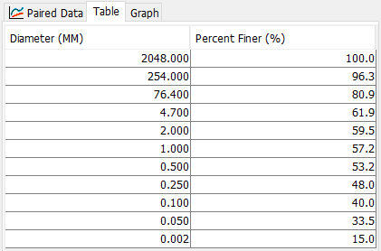
- Manually enter the gradation curve data.
- Select the Table tab.
- Enter the soil diameters from largest to smallest or smallest to largest.
- Enter the corresponding percent finer for each soil diameter.
- In this case, the more detailed gradation curve with more soil categories was used.
- Select the appropriate Grade Scale to be used within each basin model in HEC-HMS.
Developing a Gradation Curve with Physical Soil Sample Data
In this option, gradation curves are developed based on the availability or collection of data from physical soil sampling. For subbasin elements, it should be noted that these gradation curves do not affect the computation of the bulk sediment discharge. They are used to specify the proportion of the total sediment discharge to each grain size class, shown in the sediment load by grain class results. For reach and reservoir elements, soil samples specific to those elements should be used to define the gradation curves.
Existing soil information from the gSSURGO database can be used to guide representative physical sample locations. For example, if a common soil type is identified on a soil map, one physical sample can be collected within that soil type to represent the gradation for the HEC-HMS subbasins that fall within that soil type area. Physical soil sampling should include bulk samples from 1) the surface of subbasins (subbasin elements), 2) channel bed surface (reach elements), or 3) reservoir bed surface (reservoir elevations). Depending upon the size of the soil particles, after both bulk sampling and pebble count are performed, two gradation curves from both methods need to be combined into a single gradation curve (composite gradation curve), based on the procedures developed by Bunte and Abt (2001). Bulk samples should be collected in accordance with ASTM D6913, since as the maximum field particle size increases so does the required minimum dry mass that needs to be collected. Bulk soil samples should be analyzed in a soil lab to get the grain size distribution curves. The traditional sieve analysis (ASTM D6913) is typically performed for sand and coarser material, while finer materials (silt and clay) are assessed using a hydrometer test (ASTM D7928), a pipette test (Olmstead et al. 1930), or a laser diffraction (Konert and Vandenberghe 1997).
References
ASTM D6913. "Standard Test Methods for Particle-Size Distribution (Gradation) of Soils Using Sieve Analysis." D6913/D6913M-17, American Society for Testing and Materials, International, West Conshohocken, PA.
ASTM D7928 (2017a). "Standard Test Method for Particle-Size Distribution (Gradation) of Fine-Grained Soils Using the Sedimentation (Hydrometer) Analysis." ASTM D7928-17, American Society for Testing and Materials, International, West Conshohocken, PA.
Bunte, K., and Abt, S. R. (2001). "Sampling Surface and Subsurface Particle-Size Distributions in Wadable Gavel- and Cobble-Bed Streams for Analyses in Sediment Transport, Hydraulics, and Streambed Monitoring." General Technical Report RMRS-GTR-74, F. S. U.S. Department of Agriculture, Rocky Mountain Research Station, ed.Ft. Collins, CO.
Konert, M., and Vandenberghe, J. (1997). "Comparison of laser grain size analysis with pipette and sieve analysis: a solution for the underestimation of the clay fraction." Sedimentology, 44, 523-535.
Olmstead, L. B., Alexander, L. T., and Middleton, H. E. (1930). "A Pipette Method of Mechanical Analysis of Soils Based on Improved Dispersion Procedure." Technical Bulletin No. 170, U.S. Department of Agriculture, Washington D.C.