Calibrate the Deficit and Constant Basin Model to Observed Annual Maximum Flows

Return to Calibrate the Soil Moisture Accounting Basin Model for a Single Water Year

Last Modified: 2023-03-11 20:05:40.893

HEC-HMS Version

HEC-HMS version 4.11 was used to create this tutorial. You will need to use HEC-HMS version 4.11, or newer, to open the project files.

Project Files

If you are continuing from Calibrate the Soil Moisture Accounting Basin Model for a Single Water Year, you may continue to use your current project files. Otherwise, download the initial project files here:

EF_Russian_River_Task_3_Initial.zip

1. Notice the subbasin element in the EF Russian DC 1951-2010 basin model uses the Deficit and Constant loss method. View the Deficit and Constant loss parameters in the component editor by highlighting the EF Russian 20 subbasin in the watershed explorer, then select the loss tab in the component editor (Figure 1).
   
2. The focus of this calibration is to reproduce annual maximum flow values at gage location Calpella for the 60 year analysis period. Flow peaks are most sensitive to the Constant Rate parameter for the Deficit and Constant loss method. The Constant Rate represents the infiltration capacity of the soil when the soil is saturated. Think about how adjusting the Constant Rate parameter might affect peak runoff. For the actual Russian River study, the hydrology model was calibrated to average monthly water volumes and average daily flows prior to calibrating to annual maximum flows. The basin model you will begin with in this task has calibrated canopy, loss, and baseflow parameters that reproduce observed monthly water volumes and average daily flows. The next step will be to adjust the Constant Rate parameter to reproduce observed annual maximum flow peaks. The parameter value for Constant Rate has been initially set based on a soils analysis in a GIS and will be the focus for adjustment during calibration.
3. A simulation run named WY 1951-2010 DC has been created that incorporates the basin model EF Russian DC 1951-2010. Compute the simulation run WY 1951-2010 DC to establish a starting point for calibration.
4. When HEC-HMS completes a simulation run, output is written to a DSS file in the HMS project folder (…\EF_Russian_River). The default name for the output DSS file is the name of the simulation run. When the compute is complete, browse to the output DSS file for the deficit and constant simulation run. Open the DSS file WY_1951_2010_DC.dss in HEC-DSSVue (you can download DSSVue from https://www.hec.usace.army.mil/software/hec-dssvue/downloads.aspx).
5. You will use the Math Functions tool in HEC-DSSVue to generate an annual maximum flow series. For this task you are analyzing flow at the Calpella Gage. Select the DSS record //CALPELLA GAGE/FLOW/01DEC1949 – 01DEC2010/1HOUR/RUN:60YR DC/ (Figure 2).
   
6. With the record selected, open the Math Functions tool from the Tools | Math Functions menu or by clicking the  button. In Math Functions dialog, open the 'Time Functions' tab. Specify the following:
   1. Operator: Min/Max/Avg/… Over Period
   2. Function Type: Maximum for Period
   3. New Period Interval: Water Year
   4. Check "Save as Irregular Interval (get time of occurrence)" box
   5. Block Size: IR-YEAR
      Figure 3 shows these options selected in the Math Functions tool. Click Compute. When the compute is complete 'Compute Complete' will be displayed in the lower left corner of the Math Functions dialog.
      
   6. Calibration is an iterative process. When calibrating it is helpful to keep track of model runs. Use Save As (File | Save As or the  button) to save the record with a distinguishable name. In this case, the model DSS record can be renamed with F-Part RUN1 (Figure 4). Subsequent runs can be named in like manner.
      
   7. Select Yes when prompted to update the catalog. Close the Math Functions Dialog.
7. You will now copy the annual maximum flow data into Excel to analyze. An Excel spreadsheet with the observed annual maximum flow series is available at the beginning of this page. Open the spreadsheet "EF Russian River Compare.xlsx." Select the annual maximum flow series DSS record created in the previous step: //CALPELLA GAGE/FLOW/01JAN1950 – 01JAN2010/IR-YEAR/RUN1/. Tabulate the DSS record using either Display | Tabulate or the  button. Select tabulated records for WY 1951-2010 (Note: WY 1951 begins on October 1, 1950 – this will be the second record in the table). Select by click and dragging your mouse or using the key combination Ctrl + Shift + End (Figure 5). Copy the selection and paste into the "Computed" column in the spreadsheet ("DC" tab). It is good practice to double-check that the number of records corresponds to the number of events in the period of analysis when pasting to Excel (In this case COUNT = 60; Figure 6).
   
   
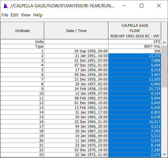
8. The objective of this calibration is for computed annual maximum flows to reproduce observed annual maximum flows. On average there should be a 1:1 relationship between computed and observed values. A scatter plot has been provided in the spreadsheet to evaluate the relationship between computed and observed values (Figure 6). A best fit line with slope intercept set equal to zero is plotted next to a line with slope = 1 to provide a graphical indication of fit. The equation of the best fit line provides a quantifiable indication of fit. The coefficient of determination (R²) indicates the how close the data fit the regression line. In this case the slope of the best fit line is really close to 1. This model can be considered calibrated to annual maximum flows. Try additional constant loss rate values to determine the optimal value for simulating peak flows. 

Project Files

Download the final project files here:

EF_Russian_River_Task_3_Final.zip

Continue to Calibrate the Soil Moisture Accounting Basin Model to Observed Annual Maximum Flows