Download PDF
Download page Validate an HEC-HMS Model using Flow Frequency.
Validate an HEC-HMS Model using Flow Frequency
Return to Calculate Performance Metrics for Daily Flows
Last Modified: 2024-09-05 18:03:13.263
HEC-HMS Version
HEC-HMS version 4.12 was used to create this tutorial. You will need to use HEC-HMS version 4.12, or newer, to open the project files.
HEC-SSP version 2.3 was used to create this tutorial.
Project Files
If you are continuing from Calculate Performance Metrics for Daily Flows you may continue to use your current project files. Otherwise, download the initial project files here:
 PeakFlow_WY_1951_2010_SMA.dss
 EF_Russian_River_SSP_Initial.zip
Introduction
Flow frequency analysis is a common part of hydrologic studies and design. Flood frequency analysis estimates the probability that annual maximum flows will exceed a particular value. A flow frequency curve is a plot of flow vs. exceedance probability for a given location. Bulletin 17C (2019) provides guidance for a standard approach for determining flow-frequency. HEC-SSP provides automated tools for Bulletin 17C flow frequency analysis provided annual maximum flow data.
England, J.F., Jr., Cohn, T.A., Faber, B.A., Stedinger, J.R., Thomas, W.O., Jr., Veilleux, A.G., Kiang, J.E., and Mason, R.R., Jr., 2018, Guidelines for determining flood flow frequency—Bulletin 17C (ver. 1.1, May 2019): U.S. Geological Survey Techniques and Methods, book 4, chap. B5, 148 p., https://doi.org/10.3133/tm4B5.
In this task you will compare flow-frequency curves computed from HEC-HMS model results and from observed data. An HEC-SSP project has been started that will allow you to perform flow frequency analysis in HEC-SSP. HEC-SSP can be downloaded here: HEC-SSP Downloads (army.mil).
- The first step is to import the annual maximum flow series created in Calibrate the Soil Moisture Accounting Basin Model to Observed Annual Maximum Flows. The annual maximum peak flows are contained in the PeakFlow_WY_1951_2010_SMA.dss file provided to you above.
- Open the HEC-SSP project. Open the Data Importer by selecting Data | New | Traditional Import.
- Name: provide a name for the data, Calpella HMS Results.
- Data Type: Time Series.
- Location: HEC-DSS.
- DSS File: Select the DSS file that contains annual maximum flow record (…/PeakFlow_WY_1951_2010_SMA.dss).
- DSS Pathname: Select annual maximum flow DSS record by double-clicking: //CALPELLA GAGE/FLOW/21JAN1951 - 20JAN2010/IR-YEAR/RUN:WY 1951-2010 SMA - WY_final/. The figure below shows these options selected in the Data Importer.
- Click Import to Study DSS File.

- The imported dataset should now be visible in "Data" node of the Study Explorer.
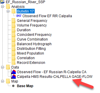
- After the data is imported, the next step is to create a Bulletin 17 analysis on the annual maximum flow data. In HEC-SSP open the Bulletin 17 editor by selecting Analysis | New | Bulletin 17 Analysis. Specify the following:
- Name: Provide a name for the analysis, Calpella HMS Results.
- Flow Data Set: Select the annual maximum flow data set (data that was imported in previous step, Calpella HMS Results-CALPELLA GAGE-FLOW).
- Choose Method 17C EMA.
- The following figure shows these options selected in the Data Importer. Since we are not adding any historic information (EMA Data tab), click Compute at the bottom of the window. A message window will open to notify when the compute is complete.

- Once the compute is complete, a plot of the flow frequency curve can be viewed by clicking the Plot Curve button at the bottom of the Bulletin 17 Editor.

- The computed flow frequency curve can be viewed in tabular form by selecting the Tabular Results tab in the Bulletin 17 Editor.

- A spreadsheet has been prepared that will allow you to compare the computed flow frequency curve to the observed. Open the spreadsheet EF Russian River Frequency.xlsx provided at the beginning of this page.
- Select the computed curve values in the HEC-SSP Bulletin 17 Editor by click and dragging your mouse or by clicking in the top data cell and using the key combination Ctrl + Shift + End. Copy the selection and paste into the "Computed" column in the spreadsheet "Calpella Probability(ZData)".

- Next, copy annual maximum flow values. Right click on the imported dataset in Study Explorer of HEC-SSP. On the right-click menu select Tabulate.

- Select tabulated records for WY 1951-2010. Select by click and dragging your mouse or using the key combination Ctrl + Shift + End.

- Copy the selection and paste into the "CALIBRATED" column in the spreadsheet "Calpella Probability(ZData)" tab.

- Sort the data in Excel by selecting the data and clicking the
 button (largest to smallest) on the "DATA" ribbon. Select "Continue with the current selection" when prompted with the sort warning.
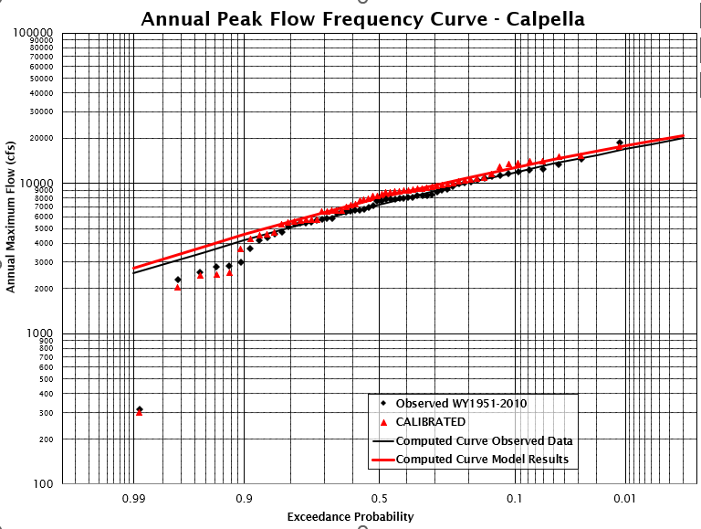
- Select the "Calpella Historic Plot" tab to view the computed flow-frequency curve plotted against the observed flow-frequency curve.
- Select the computed curve values in the HEC-SSP Bulletin 17 Editor by click and dragging your mouse or by clicking in the top data cell and using the key combination Ctrl + Shift + End. Copy the selection and paste into the "Computed" column in the spreadsheet "Calpella Probability(ZData)".
For rare flood events it is important for the high flow end of the flow frequency curve to reproduce the observed. In this case the model performs well across the spectrum of flows but while fine tuning during calibration, emphasis was placed on the high flow end of the curve rather than middle or low flow portions. There does appear to be a bias in the HEC-HMS results. Generally, the HEC-HMS peak flows are larger than the observed peak flows. You could improve the HEC-HMS results by reducing the Clark storage coefficient parameter, or the GW 1 fraction parameter.
Download the final project files here:
This concludes the Calibrating a Continuous Simulation Model tutorial.