Download PDF
Download page Calibrate a Basin Model to Event 2.
Calibrate a Basin Model to Event 2
Last Modified: 2025-01-29 19:03:43.045
Software Version
HEC-HMS version 4.13 beta 4 was used to create this example. You can open the example project with HEC-HMS 4.13 or a newer version.
Download the Initial project file here:
 Initial_Event2_Calibration.zip
Overview
Now that you've calibrated one basin model, use your newfound talents to calibrate another event. It is good practice to calibrate your hydrologic model to more than one storm event. Model parameters are not static values that exist without variability. On the contrary, given the heterogeneity that exists within the watershed basin with differing soil types, changes in land use and vegetation as well as differing antecedent soil conditions, model parameters and their associated watershed response are expected to change for different storm events. This is another important reason to understand how your model predictions will be used and to tailor your calibration events to reflect what will be predicted. For example, if you are interested in estimating the 1% annual chance exceedance event, you'll want to look at storm events that produced high flows and not storms that produce average flows.
Another large storm event within the Mahoning watershed occurred in April 1994. In this tutorial, you'll use what you learned in the last lesson to calibrate Mahoning Creek watershed. A meteorological model has already been set up for you and you will not need to make any adjustments. You'll notice that the Meteorological method uses Gage Weights method rather than Gridded Precipitation. In many cases, gridded precipitation will be harder to come by as you go further back in time. In such cases, point rain gages may be the only rainfall boundary available for calibration.
Initialize and Calibrate Parameters
- Download the workshop provided and open up the Punx.hms project
You'll see a new basin model called Apr1994 under the Basin Model folder. Model parameters for each subbasin are left empty. How will you go about initializing your subbasin parameters?
Consider using the calibrated parameters from the previous effort since this is your current best estimate.
Subbasin Deficit and Constant Clark UH Linear Reservoir Initial Deficit (in) Constant loss (in/hr) Tc (hr) R (hr) GW1 Coefficient (hr) GW2 Coefficient (hr) East Branch Mahoning 1.8 0.060 10.7 10.9 44 131 Stump Creek 1.8 0.060 13.4 13.5 55 164 Mahoning Creek Local 1.8 0.060 15.7 15.9 64 193 - Enter your estimate for Deficit and Constant loss
- Enter your estimate for Clark Unit Hydrograph
- Enter your estimate for Linear Reservoir Baseflow
- Run the simulation
- After you've initialized all model parameters, select Apr1994 in the simulation runs list and run the simulation
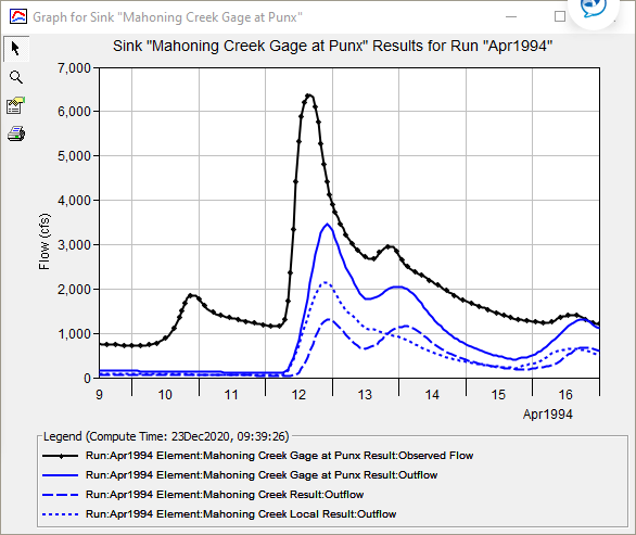
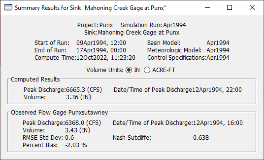
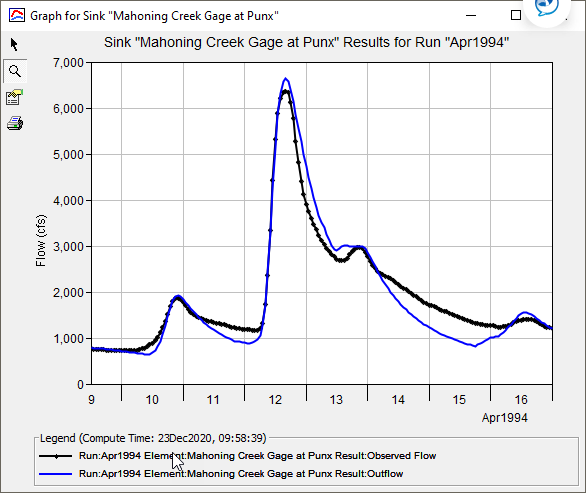
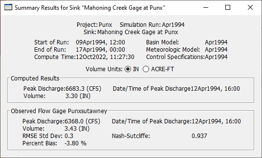
In the Results tab, click on the Apr1994 simulation and expand the Outlet element. Select the Graph and Summary Results. How do the results look?
Even using calibrated parameters, you can see the simulated results significantly under predict the observed results. This is a good example on how antecedent conditions can affect the watershed response. Also, initial conditions are event specific. Initial losses and baseflow should be set for each event.

- Calibrate your model
- Calibrate the model on your own using what you've learned in the past few tutorials. If you get stuck, a calibration solution is provided for you below. Additionally, here are some more guiding principals for calibration
Adjust one parameter at a time.
Adjust parameters which you have the least amount of confidence with their initial estimates.
Look for evidence to support or motivate parameter adjustments.
Beware of the natural tendency to want to change only the parameters that have a large impact. It can lead you to make unrealistic changes to several parameters which individually have little impact but collectively have a large impact.
Manual calibration is useful for identifying parameters that have a large impact on results. This can be used to wisely allocate your time. Consider going back and spending additional time using physically based methods to estimate just these parameters.
- Calibrate the model on your own using what you've learned in the past few tutorials. If you get stuck, a calibration solution is provided for you below. Additionally, here are some more guiding principals for calibration
Solution
- Adjust GW 1 and GW 2 Initial Baseflow
- Using one of the guiding principals, we have a lot of uncertainty surrounding the initial baseflow value. This is clearly seen when comparing the observed hydrograph with the simulated hydrograph
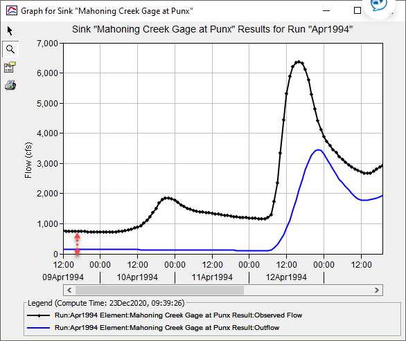
- Increased GW 1 Initial to 2 CFS/MI2 and GW 2 Initial to 3 CFS/MI2. This improved the initial discharge at the beginning of the simulation
- Using one of the guiding principals, we have a lot of uncertainty surrounding the initial baseflow value. This is clearly seen when comparing the observed hydrograph with the simulated hydrograph
- Adjust Deficit and Constant Loss
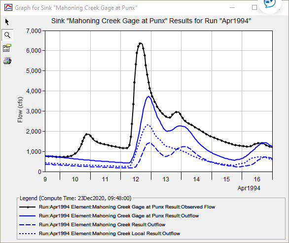
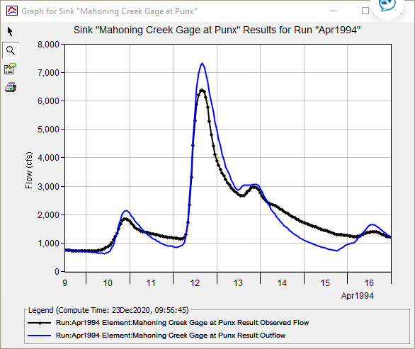
- The observed hydrograph shows runoff from the storm event around the middle of the 10th of April but simulation results do not show a runoff response suggesting the initial deficit value may be too large. The simulated volume in the Summary Results is lower than the observed volume for the simulation period. Reduced Initial Deficit value to 0.4 inches for all subbasins. This improved the initial runoff response
- The observed hydrograph shows runoff from the storm event around the middle of the 10th of April but simulation results do not show a runoff response suggesting the initial deficit value may be too large. The simulated volume in the Summary Results is lower than the observed volume for the simulation period. Reduced Initial Deficit value to 0.4 inches for all subbasins. This improved the initial runoff response
- Adjust Clark Unit Hydrograph
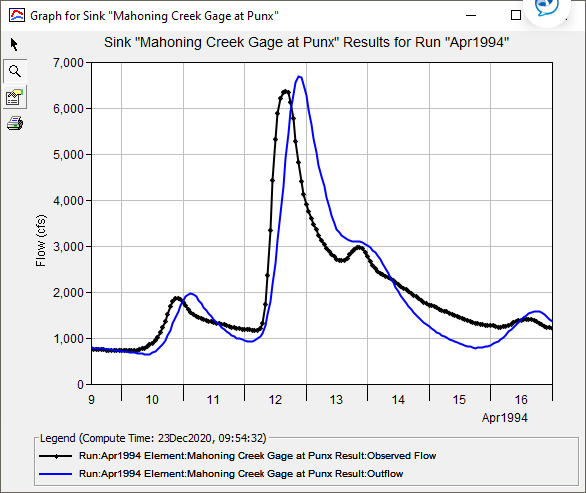
- The simulated hydrograph peak occurs a number of hours later compared to the observed hydrograph event. The Summary Results shows the simulated hydrograph peaks 5 hours later
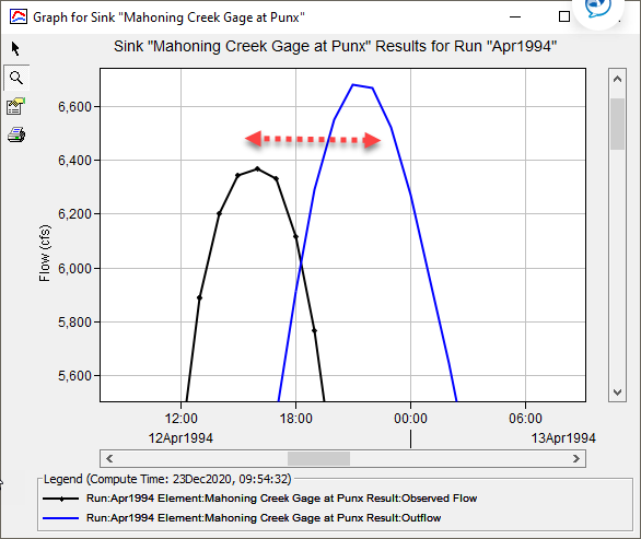
- Reduced Time of Concentration for all subbasins by a factor of 0.4. This improved the timing of the simulated hydrograph

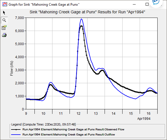
- The hydrograph shape matches reasonably well. Adjust the Clark storage coefficient by multiplying the storage coefficient by a factor of 1.1 for all subbasins

- The simulated hydrograph peak occurs a number of hours later compared to the observed hydrograph event. The Summary Results shows the simulated hydrograph peaks 5 hours later
- Minor changes to improve simulation results
- Went back to Deficit and Constant loss method and increased constant loss to 0.075 in/hr.
- Increased GW 1 and GW 2 Coefficients by a factor of 1.4
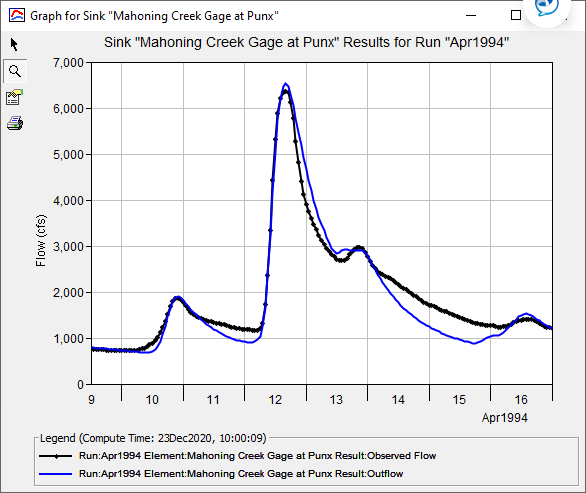
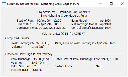
- Went back to Deficit and Constant loss method and increased constant loss to 0.075 in/hr.
- Adjust GW 1 and GW 2 Initial Baseflow
Download the final project file here:
Final_Event2_Calibration.zip
Questions
Which parameters had the largest impact to the calibration?
The initial baseflow and initial deficit appear to be very sensitive parameter. As mentioned, this shows the variability that exists with your antecedent conditions and how it can affect watershed response.
How do your April 1994 calibrated parameters compare to the Sept 2018? Is one better than the other?
Event Subbasin Deficit and Constant Clark UH Linear Reservoir Initial Deficit (in) Constant loss (in/hr) Tc (hr) R (hr) GW1 Coefficient (hr) GW2 Coefficient (hr) Sep-18 East Branch Mahoning 1.8 0.060 10.7 10.9 44 131 Apr-94 0.4 0.075 4.3 12.0 61 184 Sep-18 Stump Creek 1.8 0.060 13.4 13.5 55 164 Apr-94 0.4 0.075 5.4 14.9 76 229 Sep-18 Mahoning Creek Local 1.8 0.060 15.7 15.9 64 193 Apr-94 0.4 0.075 6.3 17.5 90 270 As noted in the first question, the largest changes were seen in the initial baseflow and initial deficit. The April 1994 event hydrograph had a much lower time of concentration showing a quicker runoff response than the September 2018 hydrograph, likely due to the differences in antecedent conditions. The watershed basin appears to have been nearly saturated prior to the April 1994 event given the higher baseflow and low initial deficit (more water in the channel will result in higher velocities and shorter time of concentration values). If you have confidence in your model boundary conditions, set up, and model results, the model parameters are of equal importance and best reflect the state of the watershed for that storm event. If you are not confident in your boundary conditions or calibration results, you may want to consider calibrating to another storm event.
How did your calibration effort go? What NSE values did you receive?
Answers will vary
This tutorial concludes the Calibrating a Simple Basin Model tutorial group.