Download PDF
Download page Task 1: Reservoir Volume Reduction Modeling with Outflow Structure Routing Method (Elevation-Area).
Task 1: Reservoir Volume Reduction Modeling with Outflow Structure Routing Method (Elevation-Area)
HEC-HMS version 4.14 Beta 1 was used to develop this tutorial.
Download the DSS data file here - Reservoir_Data.dss
Overview
This example illustrates steps to develop a basic HEC-HMS reservoir volume reduction model from scratch using existing field data. You will summarize the model parameters from the given field data set and choose appropriate input parameters for the reservoir sedimentation simulation. Data used in the development of this model can be found in the attached Reservoir_Data.dss file (see the Introduction to Reservoir Volume Reduction Methods page for an overview of how this data was derived).
Develop the Model
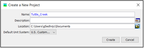
- Create a new HEC-HMS project with HEC-HMS version 4.10 or greater by selecting File | New.
- Name the project Tuttle_creek
- Set the proper project Location.
- Set the Default Unit System to US Customary.
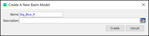
- Create a new basin model by selecting Components | Create Component | Basin Model.
- Name the basin model Big_Blue_R.
- Name the basin model Big_Blue_R.
- Select the Basin Models folder to expand the Watershed Explorer.
- Select Big_Blue_R Basin Model.
- Click the source creation tool icon
 in the components toolbar.
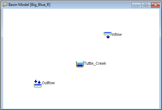
 - Click on the basin map to create a source element and name the source element Inflow.

- Switch to the reservoir creation tool icon
 in the components toolbar.
 - Click on the basin map to create a reservoir element and name the reservoir element Tuttle_Creek
- Switch to the sink creation tool icon
 in the components toolbar.
 - Click on the basin map to create a sink element and name the sink element Outflow.
- The elements should be placed as shown in the figure below.
- Connect the elements into a hydrologic network as shown in the figure below. Click on the arrow button (left of the creation tools)
 . Then, right click on Inflow source element and select the Connect Downstream option. Use the mouse to identify the reservoir element Tuttle_Creek as the downstream element. A connection line is drawn to show the elements are connected. In the same way connect the Tuttle_Creek element to the Outflow element.
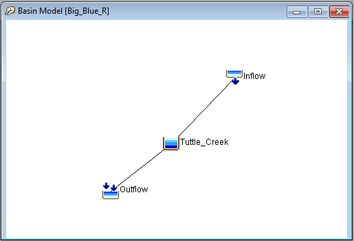
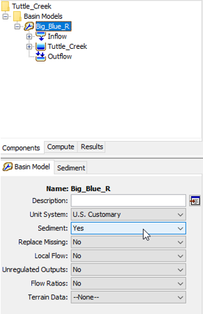
- Select the Basin Model (Big_Blue_R) and select Yes for the Sediment option in the Basin Model Tab as shown below.
- Select the Inflow source element.
- Select Discharge Gage for the Flow Method.
- Select Specified Load for the Sediment Method.

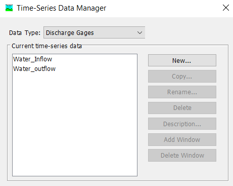
- Go into the Components | Time-Series Data Manager to create time-series for the observed data.
- Under Data Type select Discharge Gages and create two new time-series named Water_inflow and Water_outflow.
- Under Data Type select Stage Gages and create a new time-series named Lake_elevation.
- Under Data Type select Sediment Load Gages and create a new time-series named Sediment_inflow.
- Under Data Type select Discharge Gages and create two new time-series named Water_inflow and Water_outflow.
- Select the Components | Paired Data Manager menu option.
- Under Data Type select Elevation-Area-Functions and create a new paired dataset named 1957_survey.
- Select Data Type: Diameter-Percentage Function and create a new paired dataset named Inflow_gradation.

- Link the newly created datasets to the HEC-DSS file Reservoir_Data.dss.
- Expand the Time-Series Data | Discharge Gages folder and select Water_Inflow.
- Under Data Source select Single Record HEC-DSS.
- Under the DSS Filename click the File Path Chooser and navigate to where the Reservoir_Data.dss file is saved as shown below (make sure you save this file to the data folder inside the HEC-HMS project directory).
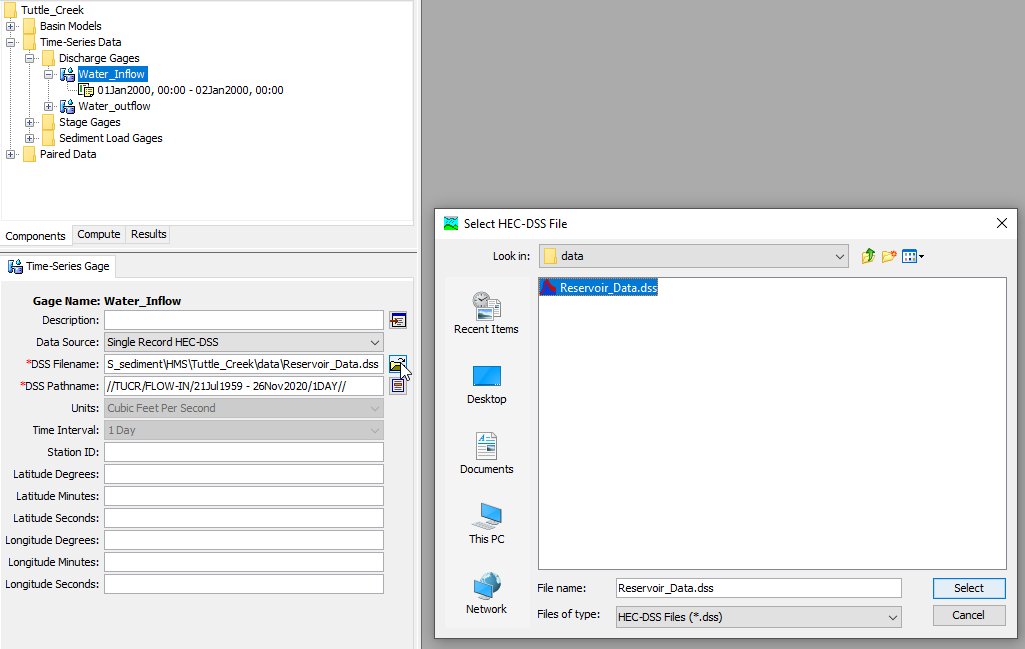
- Under the DSS Pathname select the dss path that has FLOW-IN in the Part C as shown below.

- Repeat the above steps for the Water_outflow timeseries, selecting the FLOW-OUT for the Part C pathname.
- Expand the Time-Series Data | Stage Gages folder and select Lake_elevation.
- Set the DSS Filename to the Reservoir_Data.dss file and the DSS Pathname to the pathname that has ELEV for the Part C.
- Expand the Time-Series Data | Sediment Load Gages folder and select Sediment_inflow.
- Set the DSS Filename to the Reservoir_Data.dss file and the DSS Pathname to the pathname that has SEDIMENT LOAD for the Part C.
- Expand the Paired Data | Elevation-Area Functions folder and select 1957_Survey.
- Set the DSS Filename to the Reservoir_Data.dss file and the DSS Pathname to the pathname that has ELEVATION-AREA for the Part C.
- Expand the Time-Series Data | Discharge Gages folder and select Water_Inflow.
- Enter the sediment inflow gradation.
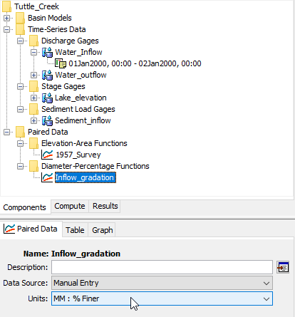
- Expand the Paired Data | Diameter-Percentage Functions folder and select Inflow_gradation.
- Under Data Source select Manual Entry.
- Under Units select MM: % Finer as shown below.
- In the Table tab, enter the values shown below.

- Assign parameters to the Inflow element.
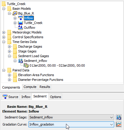
- Select the Inflow source element and go into the Inflow tab.
- Assign Water_Inflow as the Discharge Gage.
- Click the Sediment tab and specify Sediment_inflow for the Sediment Gage and Inflow_gradation for the Gradation Curve.
- Select the Inflow source element and go into the Inflow tab.
- Assign reservoir parameters to the Tuttle_Creek reservoir element.
- Under the Basin Model folder, select the Tuttle_Creek reservoir element.
- In the Reservoir tab, select Outflow Structures for the Method.
- Select the 1957_Survey dataset for the Elev-Area Function.
- Set the Initial Condition to Elevation and for the Initial Elevation type in 1030 feet.
- Under Release select Yes.
- Select the Yes option for the Sediment option.
- The Reservoir tab for Tuttle_Creek should look like the figure below.

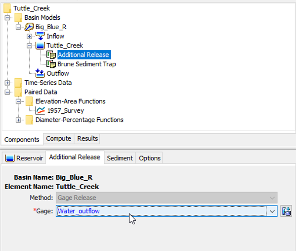
- Expand the Tuttle_Creek reservoir element, click on the Additional Release tab, and select Water_outflow for the Gage release.
- Click on the Sediment tab in the Tuttle Creek reservoir element to enter parameters for computing the reservoir trapping efficiency and sediment deposition shape. .
- Select the Brune Sediment Trap option for the Sediment Method.
- Enter 1,560,000 AC-FT for the Annual Inflow Volume (this represents the average annual inflow of water into the reservoir).
- Enter 1075 FEET for the Capacity Elevation. The capacity elevation should approximate the average trapping efficiency within the reservoir.
- Enter 100 for Constant A, 7.71 for Constant B. These are the Brune Curve coefficients for computing reservoir trapping efficiency.
- Select Yes for the Reservoir Capacity Method (this will cause HMS to update the elevation-area and elevation-volume tables throughout the simulation).
- Select V-Shape for the Clay Deposition Shape.
- Select Elongated Taper for the Silt, Sand, and Gravel Deposition Shape.
- Enter 0.0 for Sediment Porosity.
- Select the Rubey option for the Fall Velocity method.
- Select the None for the Hindered Settling Velocity method.

- Go to the Options tab in the Tuttle_Creek reservoir element and select Lake_elevation for the Observed Pool Elevation.
- Go into the Components | Meteorological Model Manager and create a new meteorological model named 1959_to_2009. No meteorological data needs to be entered because gaged flow data is being used for the reservoir inflow. However, a meteorological model is needed to run a simulation.
- Select the meteorological model just created and under the Basins tab, select Yes to include the Big_Blue_R basin model. Set all the modeling options in the meteorologic model to None.

- Go into the Components | Control Specification Manager and create a new control specification named 1959_to_2009.
- Click on the control specification just created and enter the values shown below.

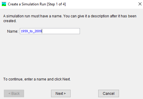
- Go into the Compute | Create Compute | Simulation Run window and create a new simulation run named 1959_to_2009. Select Big_Blue_R for the basin model, 1959_to_2009 for the meteorological model and 1959_to_2009 for control specifications.
- Compute the simulation run: A simulation run must be selected before it can be computed. The toolbar includes a selection list that shows all of the simulation runs that have been created in the project. Click on the selection list and choose RUN: 1959_to_2009. Once a simulation run has been selected, click on the Compute button
 , immediately to the right of the selection list, to perform the compute. A compute progress window will open to show the advancement of the simulation. The simulation may abort if errors are encountered. If this happens, read the messages and fix any problems; then compute the simulation run again. Close the progress window when the run computes successfully. Estimated runtime should be less than one minute depending on your processor speed.
- After the simulation is complete, the reservoir water surface elevation should be viewed to compare the model to observed results.
- Right click on the Tuttle_Creek reservoir element in the basin map.
- Select View Results | Graph as shown below.

- Selecting View Results | Summary Table will provide additional details on how well the modeled pool elevation matches with the observed.
Question 1: What is the Nash-Sutcliffe for the simulation?
0.902.
- View storage volume change in HEC-DSS.
- Go to your project folder using File Explorer.
- Open the output DSS file named 1959_to_2009.dss using DSSVue.
- Select the ELEVATION-STORAGE (Water) records for the first and last timesteps as shown below.

- Click on Plot to view how the elevation-storage curve changes over the simulation period.

- The total storage volume lost from the reservoir can be computed by subtracting the last storage curve from the first.
- Using the same two datasets selected in the previous step, select the Tabulate tool.
- Using Excel or a calculator, subtract the final storage from the starting storage at elevation 1159.0.
Question 2: What is the total storage volume lost from the lake due to sedimentation?
179,549 acre-ft.