Download PDF
Download page Calibrating Gridded Snowmelt: John Day River Watershed.
Calibrating Gridded Snowmelt: John Day River Watershed
Disclaimer: The United States Army Corps of Engineers has granted access to the information in this model for instructional purposes only. Do not copy, forward, or release the information without United States Army Corps of Engineers approval.
Background
The U.S. Army Corps of Engineers (USACE) owns and operates a large system of dams, navigation locks, and levees within the Columbia River watershed which are critical to the normal daily activities of the nation. Additionally, close coordination with Canada is essential to operating these projects in a way that is as safe and efficient as possible. Operation of these systems provides national, regional, and local benefits that include flood damage reduction, drought impact reduction, hydropower, water supply, navigation, recreation, and environmental support as authorized by Congress.
As part of ongoing Columbia River Treaty (CRT) investigations, it was determined that hydrologic models capable of simulating the precipitation-runoff cycle were needed to better estimate flow- and volume-frequency relationships within the Columbia River watershed. The Northwestern Division (NWD) USACE requested the assistance of the Hydrologic Engineering Center (HEC) to construct, calibrate, document, and deliver these hydrologic models. HEC then partnered with multiple District and Center of Expertise personnel located throughout USACE to aid in the development of these hydrologic models.
As part of this study, an HEC-HMS model was built for the Mainstem Columbia River watershed, which encompasses the Columbia River watershed (and all tributaries) located downstream of McNary Lock and Dam and upstream Bonneville Lock and Dam. Continuous simulation processes and Geographic Information System (GIS)-derived parameters were employed within the HEC-HMS model, where possible.
Multiple large tributaries exist within this watershed. One of them is the John Day River, which will be the focus within this workshop. The location of the John Day River watershed within the larger Columbia River watershed is shown in Figure 1.
Within the previous workshop (Workshop 4: Point Snowmelt Calibration), calibrated temperature index parameters were developed for three SNOTEL stations in and around the John Day River watershed. The locations of these SNOTEL stations in relation to the John Day River watershed is shown in Figure 2. Using that information, you will now calibrate an HEC-HMS model using the gridded temperature index method. 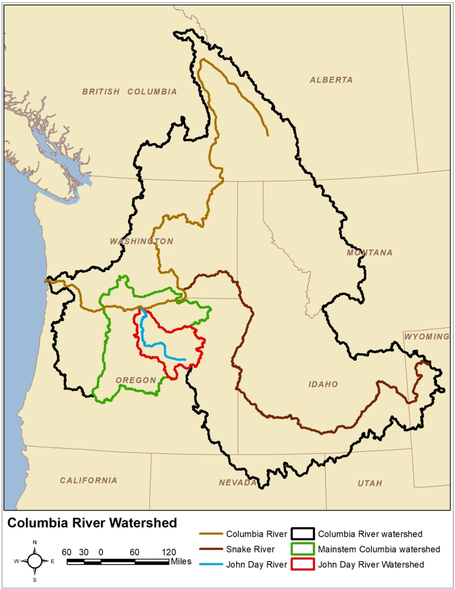
Figure 1. John Day River Watershed Location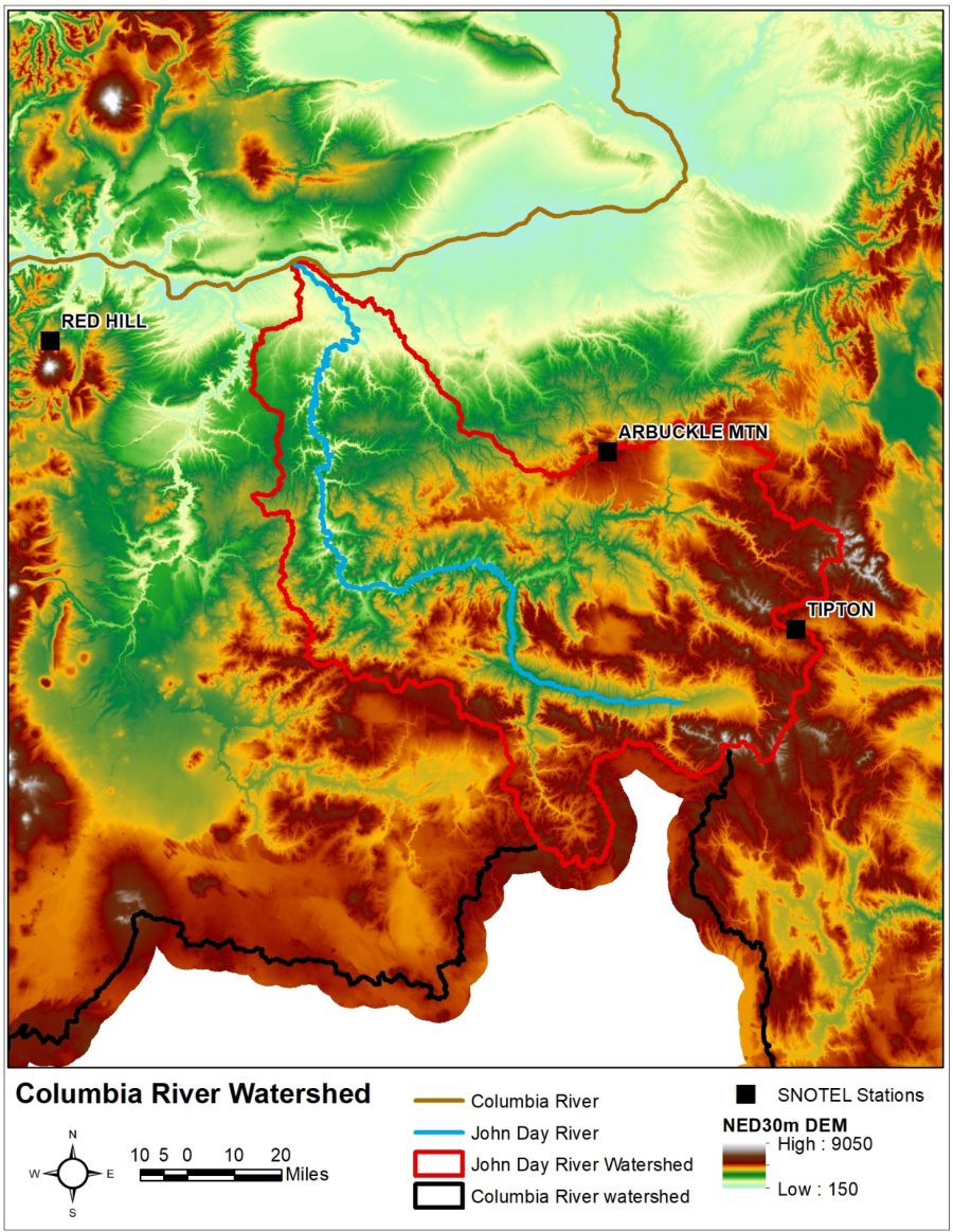
Figure 2. SNOTEL Station Locations from Previous Workshop
Objectives. In this workshop, you will gain experience using the gridded temperature index snowmelt/accumulation method within the John Day River watershed. You will refine initial temperature index parameter estimates for both the deficit constant and soil moisture accounting loss methods.
The following major tasks will serve as an outline for the workshop:
- Add temperature index parameters from the previous workshop to an existing HEC-HMS model for the John Day River.
- Compute the HEC-HMS model and compare the initial results vs observed results.
- Refine the temperature index parameters to provide better agreement between computed and observed SWE.
- Refine the linear reservoir baseflow parameters to provide better agreement between computed and observed streamflow. There will be a prize awarded to the team with the highest Nash-Sutcliffe Efficiency score at the Monument gage!
An additional task is included at the end of this workshop, if time allows.
Spend approximately 25 minutes per task to accomplish all tasks in this workshop within the time allotted.
Initial Project Files: John_Day_River.zip
Task 1: Add temperature index parameters from the previous workshop to an existing HEC-HMS model for the John Day River.
- Open the existing HEC-HMS model for the John Day River. It should be located in the "..\Workshop_5\HMS" directory.
- This model contains one basin model, one meteorologic model, one control specification, and one simulation run meant for simulating precipitation-runoff processes for water year (WY) 2011.
- Open the "GriddedSim_WY2011" meteorologic model.
- Ensure that the Precipitation, Evapotranspiration, Snowmelt, and Replace Missing options are set to Gridded Precipitation, Gridded Hamon, Gridded Temperature Index, and Set To Default, respectively.
- Click on the Gridded Precipitation method and ensure the "Precip 2010-2011" data set has been selected. A Time Shift of 0 should be used.
- Click on the Gridded Hamon method and ensure the "Temperature 2010-2011" data set has been selected. A Hamon Coefficient of 0.0065 should be used.
- Click on the Gridded Temperature Index method and ensure the "Temperature 2010-2011" data set has been selected.
- The best fit temperature index parameters from the previous workshop have been entered for each subbasin (within version 4.4, temperature index parameters can be entered at a subbasin level). Ensure the parameters shown in Table 1 are populated for each subbasin:
Table 1. Best Fit Temperature Index Parameters
Parameter | Value |
|---|---|
PX Temperature (deg F) | 33 |
Base Temperature (deg F) | 32 |
Wet Meltrate(in / deg F - Day) | 0.15 |
Rain Rate Limit (in / day) | 1 |
ATI - Meltrate Coefficient | 0.1 |
Cold Limit (in / day) | 0.2 |
ATI - Coldrate Coefficient | 0.5 |
Water Capacity (%) | 3 |
- Expand the Paired Data node in the tree and populate the "meltrate_WY2011" and "coldrate_WY2011" curves with the data shown in Table 2 and Table 3. These best fit curves were determined within the previous workshop
Table 2. Best Fit ATI-Meltrate Curve
ATI(Deg F – Day) | Meltrate(in / Deg F – Day) |
0 | 0.03 |
10 | 0.08 |
100 | 0.2 |
500 | 0.2 |
Table 3. Best Fit ATI-Coldrate Curve
ATI(Deg F – Day) | Coldrate(in / Deg F – Day) |
0 | 0 |
500 | 0.02 |
1000 | 0.02 |
Task 2: Compute the HEC-HMS model and compare the initial results vs observed results.
Now that the HEC-HMS model has been parameterized, it's time to make the first simulation and see how the initial computed results compare against observed data. When it comes to observed snow water equivalent (SWE) data, there are several options for use in hydrologic models. These data sources include snow courses, hydrometeorological gages, model output, and remotely sensed data, amongst others. Within this workshop, basin-average SWE from the National Operational Hydrologic Remote Sensing Center (NOHRSC) Snow Data Assimilation (SNODAS) model will be used to compare against the SWE computed from the HEC-HMS model. For more information regarding the NOHRSC SNODAS model and output, visit this webpage: https://www.nohrsc.noaa.gov/nsa/. The SNODAS output has already been selected for each subbasin within the John Day River HEC-HMS model.
- Compute the model by selecting the "WY2011" simulation from the compute selection drop down menu and clicking the exploding rain drop:
 .
. - Once the simulation has finished, click on the Results tab and select any subbasin element.
- For each, subbasin, there will be multiple time series available for selection. Click on the "Snow Water Equivalent" object, hold the Ctrl key, and click on the "Observed SWE" object. This will create a plot of the two selected time series. The selected time series can be shown in a separate plot window by clicking the plot button:
 .
. - Additional time series can be added to an existing plot window by left-click and holding on the time series of interest, dragging into the existing plot window, and releasing the left mouse button in the grey space around the plot.
- Marker lines can be added on either the x- or y-axis of an existing plot window by selecting the pointer (
 ), right clicking in the viewport, and selecting one of the Add Marker options.
 - Line styles/colors can be edited by clicking the Edit Graph Properties button (
 ) and selecting various plot options.
Question 1: How does computed SWE compare against observed SWE for the "JohnDayRv_S70" subbasin? Why is the computed SWE different than the observed SWE? Try plotting precipitation, temperature, computed SWE, and observed SWE in the same window (change the line styles of various curves to better visualize them). What temperature index parameters should be changed to better match observed SWE?
A plot of the precipitation (blue line in the upper viewport), temperature (red line in the lower viewport), computed SWE (blue line in the lower viewport), and observed SWE (dashed black line in the lower viewport) for the “JohnDayRv_S70” subbasin are shown in the figure below.
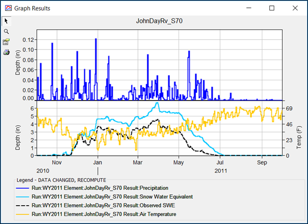
The shape of the computed SWE curve largely matches the shape of the observed SWE curve. However, the magnitude of the computed SWE curve is larger than the observed SWE curve. The computed SWE begins to deviate from the observed SWE in the beginning of December 2011. During this time, the computed SWE increases while the observed SWE decreases. Also, during this time, the basin-average temperature is very close to the initial base and PX temperatures of 32 deg F and 33 deg F, respectively. Since the shape of the two curves are very similar while the magnitudes are different, only minor changes to the base and PX temperatures are needed to match the observed data to an acceptable degree.
Question 2: How does computed SWE compare against observed SWE for the following subbasins: NFJohnDayRv_S30, JohnDayRv_S50, and JohnDayRv_S20? Which subbasin/region should receive more attention when calibrating temperature index parameters?
The initial results (computed = blue lines, observed = dashed black lines) for NFJohnDayRv_S30, JohnDayRv_S50, and JohnDayRv_S20 are shown in the figure below.
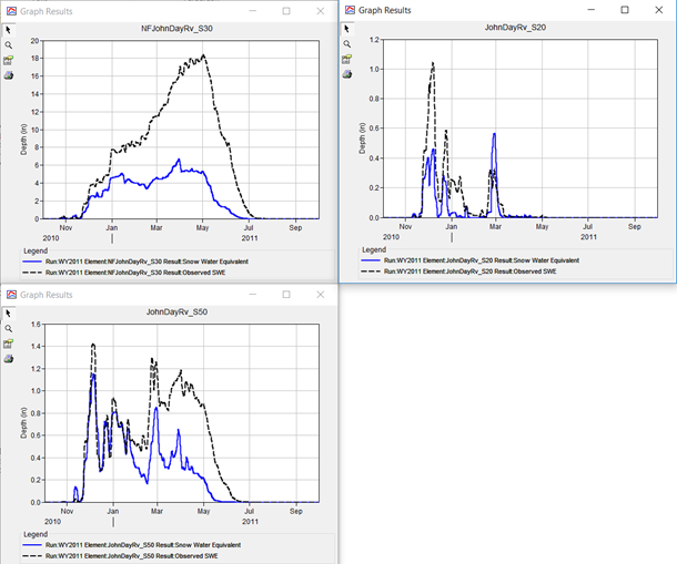
Within this figure, the computed SWE appears to not adequately match the observed SWE in any of the subbasins. However, when the magnitude of the observed SWE in each subbasin is taken into account, it’s evident that the differences within the NFJohnDayRv_S30 subbasin are much larger than the other two. The NFJohnDanRv_S30 subbasin has a peak observed SWE of approximately 18 inches compared against 1.4 and 1.0 inches of SWE within the JohnDayRv_S50 and JohnDayRv_S20 subbasins, respectively. For these reasons, much more time should be spent adjusting parameters within the NFJohnDanRv_S30 subbasin (and other similar subbasins) than the JohnDayRv_S50 and JohnDayRv_S20 subbasins.
Question 3: Using the figure in the previous answer and any other information that you can gather, provide at least two reasons why NFJohnDayRv_S30 subbasin may have larger SWE magnitudes than the other two subbasins mentioned in Question 2.
- Predominant weather patterns may be causing more precipitation to reach the NFJohnDayRv_S30 subbasin than other subbasins within the modeling domain.
- As weather systems move west to east, they will follow the terrain. As mountains are encountered, any air mass must rise. If the air mass contains moisture, precipitation will likely fall. Temperatures also tend to decrease as elevation increases. Since the NFJohnDayRv_S30 subbasin is one of the higher elevation subbasins within the modeling domain, it likely is subject to orographic influences to a larger degree than most other subbasins. Finally, when precipitation falls, the likelihood of it falling as snow is amplified due to expected decreases in temperature.
Task 3: Refine the temperature index parameters to provide better agreement between computed and observed SWE.
Now that you have completed an preliminary run and assessed the initial performance of the model when compared against observed SWE, modify the temperature index parameters within the NFJohnDayRv_S30, CamasCk_S10, MFJohnDayRv_S30, MFJohnDayRv_S20, MFJohnDayRv_S10, NFJohnDayRv_S20, NFJohnDayRv_S10, and JohnDayRv_S70 subbasins. These subbasins are highlighted in Figure 3. 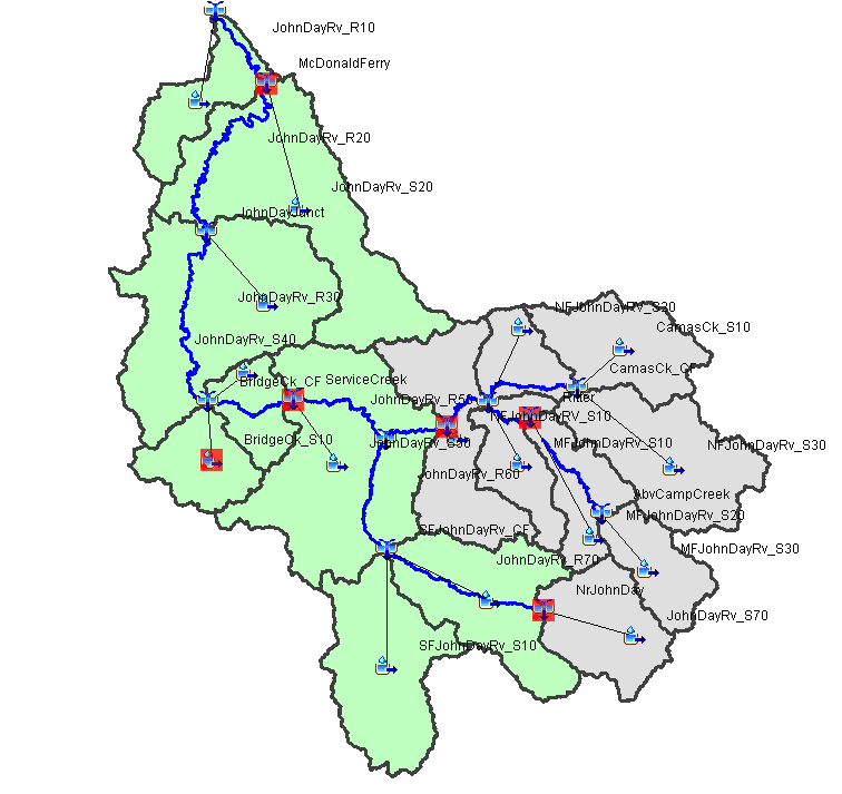
Figure 3. SWE Calibration Subbasins of Interest
Remember to think critically before you make any parameter changes. Ask yourself several questions:
- How different are the computed and observed results?
- What parameters should be changed to better align the computed and observed results?
- What magnitude change should be made (small or large)?
- Can I make the same change(s) within multiple subbasins before computing again to save myself time?
- Am I making things too complicated?
Question 4: The most common metric used to ascertain the acceptability of SWE calibration is comparing the peak computed SWE against the peak observed SWE. List at least three additional ways in which SWE calibration can be measured/determined.
Additional metrics that could be used to establish the acceptability of SWE calibration include:
- Date of peak observed and computed SWE
- Melt out date (i.e. date when SWE is completely melted) of observed and computed SWE
- Nash-Sutcliffe Efficiency (NSE)
- Ratio of the Root Mean Square Error to the Standard Deviation Ratio (RSR)
- Percent Bias (PBIAS)
Question 5: How close is "close enough" when it comes to comparing the HEC-HMS model results against the SNODAS data?
It is important to keep the goals of the study, accuracy of the computed data, and accuracy of the observed data in mind when assessing the acceptability of calibration. For instance, the “observed” SWE data used within this workshop is actually derived from another model. As such, inaccuracies within the SNODAS model processes and other data used in assimilation are present. For this reason (and others), agreement to a few inches in magnitude and a few days within the subbasins that develop the largest snowpack magnitudes is more than adequate. Also, remember that calibrating SWE is not the same thing as calibrating both SWE and streamflow. There is a give-and-take relationship between the two results and computed streamflow is a much more important parameter within the vast majority of the studies that USACE undertakes.
Question 6: When calibrating SWE within the aforementioned subbasins, did you notice any parameters that could be regionalized?
The law of parsimony states that simpler solutions to a problem tend to be more appropriate than complex solutions. In layman’s terms: the solution to a problem should be as complicated as need be to adequately solve it but no more complex. An extension of this law to the realm of hydrology would imply that simpler methods are more appropriate than complex methods. Regionalization of model processes and parameters better adheres to this law. Some important temperature index parameters that could be regionalized include:
- Range of PX and base temperature
- Base Temperature
- Wet Meltrate
- ATI-Meltrate
- ATI-Coldrate
All of these parameters can be regionalized, but may still vary a little bit throughout a region. Keep in mind that any model is a simplification of the natural world.
Task 4: Refine the linear reservoir baseflow parameters to provide better agreement between computed and observed streamflow.
Now that you have calibrated SWE within a few subbasins, compare the computed streamflow at the NrJohnDay, Ritter, and Monument gages. These gage locations are shown in Figure 4. 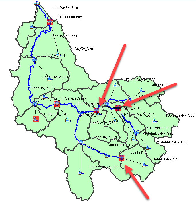
Figure 4. Streamflow Gages of Interest
Due to the use of daily precipitation (which is disaggregated to a three-hour time step) and daily average temperature, nearly all precipitation and snowmelt is infiltrated within these simulations. When combining precipitation and snowmelt rates, the sum rarely exceeds the infiltration capacity of the soils throughout the modeling domain. For instance, an infiltration rate of 0.15 inches/hour would be able to completely infiltrate the 3.6 inches of precipitation in a single 24-hour period.
As such, the calibration of linear reservoir baseflow parameters is much more important than infiltration and unit hydrograph transform parameters. Focus your efforts on these parameters and calibrate streamflow at the NrJohnDay, Ritter, and Monument gages. As you did when calibrating remember to think through any changes before making them:
- How different are the computed and observed results?
- What parameters should be changed to better align the computed and observed results?
- What magnitude change should be made (small or large)?
- Can I make the same change(s) within multiple subbasins before computing again to save myself time?
- Am I making things too complicated?
While you are calibrating the precipitation-runoff processes to the aforementioned gages, take note of the Nash-Sutcliffe Efficiency (NSE) score, which is a common metric used to ascertain goodness of fit. The Summary Results contains this information for elements that have an observed time series linked to them. The Summary Results table can be opened by selecting the element of interest and clicking on the summary table button near the top of the frame ![]() . The NSE score location is shown in Figure 5. The team with the highest NSE score at the Monument gage location will be awarded a prize. In the event of a tie, the tiebreaker will be the team with the lowest absolute value Percent Bias.
. The NSE score location is shown in Figure 5. The team with the highest NSE score at the Monument gage location will be awarded a prize. In the event of a tie, the tiebreaker will be the team with the lowest absolute value Percent Bias. 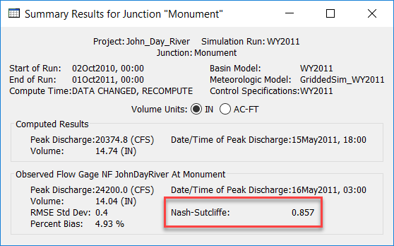
Figure 5. NSE Location
Question 7: How close is "close enough" when it comes to comparing the HEC-HMS model results against the daily streamflow data?
Comparing computed and observed peak flow, time of peak flow, and volume are common ways used to assess model calibration. However, these metrics can be incomplete in that they don’t assess model performance throughout the entirety of the hydrograph (i.e. not just the peak) and aren’t necessarily tractable. Metrics presented within Moriasi, et al (2007) represent a more complete way in which model calibration can be assessed. In general, for primary locations of interest, NSE, RSR, and PBIAS should be within the ranges defined below:
Performance Rating | NSE | RSR | PBIAS |
Very Good | 0.65<𝑁𝑆𝐸≤1.00 | 0.00<𝑅𝑆𝑅≤0.60 | 𝑃𝐵𝐼𝐴𝑆< ±15 |
Good | 0.55<𝑁𝑆𝐸≤0.65 | 0.60<𝑅𝑆𝑅≤0.70 | ±15≤𝑃𝐵𝐼𝐴𝑆<±20 |
Satisfactory | 0.40<𝑁𝑆𝐸≤0.55 | 0.70<𝑅𝑆𝑅≤0.80 | ±20≤𝑃𝐵𝐼𝐴𝑆<±30 |
Unsatisfactory | 𝑁𝑆𝐸≤0.40 | 𝑅𝑆𝑅>0.80 | 𝑃𝐵𝐼𝐴𝑆≥±30 |
Question 8: When calibrating streamflow within the aforementioned subbasins, did you notice any parameters that could be regionalized?
There are a few parameters that could be regionalized. However, the most impactful to this analysis are GW1 and GW2. These two parameters can be related to the watershed storage coefficient (Clark “R”), which itself was determined from physically-measureable characteristics of the individual subbasins. The relationship between these parameters should be maintained (to a reasonable degree) within a region.
Additional Task 1: Complete calibration of the entire John Day River HEC-HMS model.
Once you've calibrated SWE and streamflow to a few subbasins/gage locations, try calibrating the entire model. Specifically, streamflow at the Monument, ServiceCreek and McDonaldFerry gage locations are of prime importance. Prioritize model performance at these locations.
Final Project Files: John_Day_River.zip