Download PDF
Download page Calibrating Snowmelt at Gage Locations.
Calibrating Snowmelt at Gage Locations
Objectives: In this workshop, you will gain experience developing and calibrating the HEC-HMS temperature index snow accumulation and melt model. This workshop focusses on setting up a model application and calibrating it to single points, SNOTEL gages, within a watershed using observed precipitation, temperature, and snow water equivalent information. Calibrating the model will aid in understanding how individual temperature index parameters impact the simulated snow accumulation and melt. A following workshop looks at model setup and calibration using gridded precipitation and temperature datasets.
Background: For this workshop, measurements at gages within the lower Columbia River watershed will be used. Figure 1 shows the Columbia River watershed, and the three District boundaries within the Columbia River watershed. The watershed was divided into 12 basins and separate HEC-HMS models were developed for each of the basins. One of the initial steps in the HEC-HMS model development was calibration of the HEC-HMS temperature index model to SNOTEL gages. Figure 2 shows the SNOTEL gages located within the Mainstem Columbia River watershed. The gages were selected to span the watershed in both location and elevation. 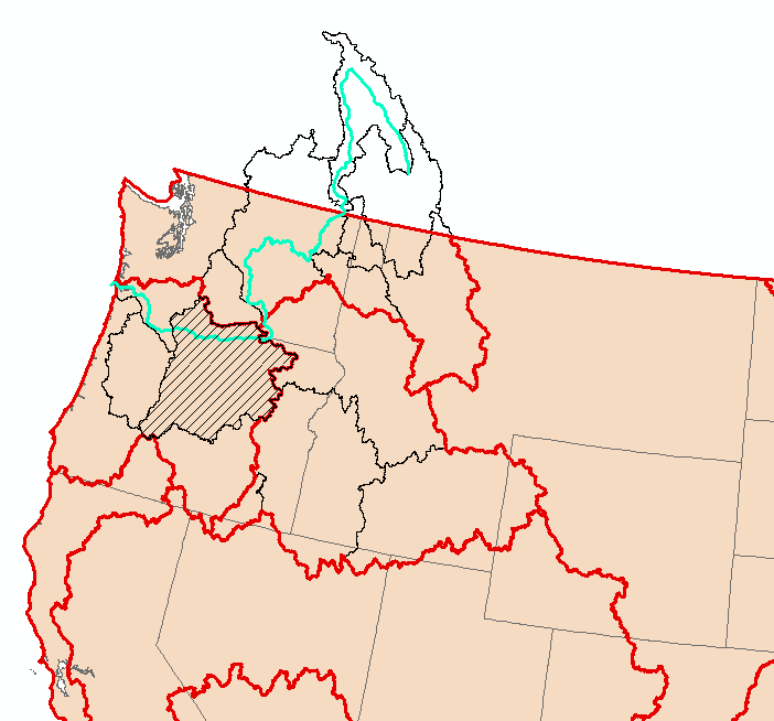
Figure 1. Columbia River watershed with District boundaries.
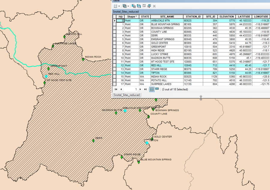
Figure 2. Mainstem Columbia River watershed with SNOTEL gages.
Tasks: The following major tasks will serve as an outline for the workshop:
- Download precipitation, temperature, and snow water equivalent data for SNOTEL gages within the Mainstem Columbia River watershed.
- Create an HEC-HMS project.
- Add time-series data to the HEC-HMS project.
- Create a Basin Model that has subbasin elements representing three SNOTEL gages.
- Create a Meteorologic Model and parameterize the precipitation and snowmelt components.
- Create a simulation for the 1997 and 1998 water years and evaluate results.
- Adjust the Temperature Index parameters to improve model results for the three SNOTEL gages.
Initial project files: maps.zip
Task 1: Download precipitation, temperature, and snow water equivalent data for SNOTEL gages within the Mainstem Columbia River watershed.
HEC-DSSVue Version 3.0 contains a plugin that will automatically download precipitation, temperature, and SWE data for selected SNOTEL gages. As shown in Figure 2, three SNOTEL gages were identified within the Mainstem Columbia River watershed. These gages are named Arbuckle Mtn, Red Hill, and Tipton, and they are located in Oregon.
- Open HEC-DSSVue and create a new DSS6 file.
- Go to Data Entry Import and select SnoTel. The SnoTel Download editor will open.
- Select the Daily data type, enter a start date of 01Oct1996 and an end date of 30Sep1998, and then select the button to Get Site List By State. Choose Oregon. The table should fill in at the bottom with all gages in the state of Oregon.
- Check the boxes to download data for the Arbuckle Mtn, Red Hill, and Tipton gages as shown in Figure 3.
- Click the Import to DSS button at the bottom of the editor. You should get a message that 22 datasets from 3 of 3 gages was downloaded. Close the SnoTel Download editor.
- Examine the downloaded records, you should notice SWE, Temperature, and Precip-Inc-Adjusted records for each of the three gages. Figure 4 shows observed SWE for the three gages. The Precip-Inc-Adjusted dataset will be used as the precipitation in HEC-HMS. This dataset was created by adjusting measured precipitation to match observed SWE volumes.
- Some changes will need to be made to the SnoTel data. With the data opened in HEC-DSSVue, select the three SWE gages and select the Tabulate option. The data for the selected records will open up in a separate window. Edit the data by selecting the Allow Editing option found under the Edit tab. While in the edit session, change the UNITS for all three gages to IN and the Type to INST-VAL. Save the edits and close the window. Select the Temperature-Air-Avg option for all three gages and tabulate the data. There will be missing data for the gages. 24Oct97 will be missing for the Arbuckle MTN gage and 21Mar98 will be missing for ALL three gages. Edit the data and fill in the missing values by interpolating between the data points around the missing values. Save the edits, close the window, and close HEC-DSSVue.
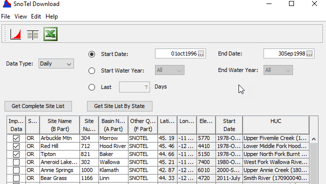
Figure 3. SnoTel data import tool in HEC-DSSVue. 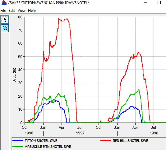
Figure 4. Observed SWE data for the Arbuckle Mtn, Red Hill, and Tipton gages.
Task 2: Create an HEC-HMS project.
- Open HEC-HMS and create a new project. Save the project to the …/Point Snow workshop directory on your computer. Make sure the Unit System is U.S. Customary.
- Copy the Subbasin and Rivers shapefiles in the …/Point Snow workshop/maps directory to the "maps" folder in your HEC-HMS project directory. (It is a best practice to keep all DSS files and background map files within your project directory.)
- Open the Program Setting editor from the Tools menu. Navigate to the Results tab and make sure the option to "Store supplemental time-series results" is selected, as shown in Figure 5. HEC-HMS will save additional output from snowmelt computations when this option is selected.
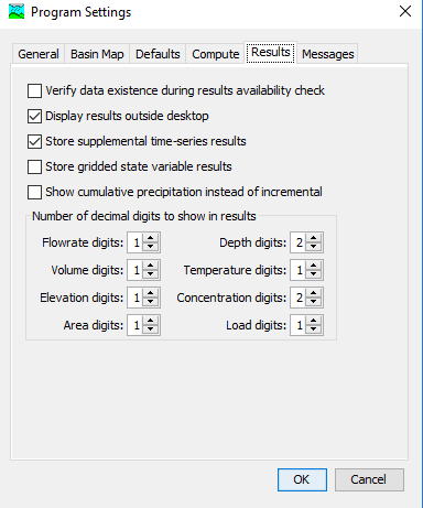
Figure 5. Store supplemental time-series results from simulations.
Task 3: Add time-series data to the HEC-HMS project.
- Using File Explorer, move the DSS file created in Task A to the "data" folder in the HEC-HMS project directory (create a data folder if one does not already exist).
- Within the HEC-HMS project, create three precipitation gages using the Time-Series Data Manager located under the Components tab. Link the gages to the correct records in the DSS file containing the SNOTEL data from the watershed explorer. Select Single Record HEC-DSS for the data source. The Precip-Inc-Adjusted dataset will be used as the precipitation in this workshop.
- Create three temperature gages using the Time-Series Data Manager. Link the gages to the correct records in the DSS file containing the SNOTEL data. Define an elevation of 5000 ft for each of the gages, and set the reference height to 32.808 ft. Use the Temperature-Air-Average records for this exercise.
- Create three SWE gages using the Time-Series Data Manager. Link the gages to the correct records in the DSS file containing the SNOTEL data.
Figure 6 shows the Time-Series Data folder in the HEC-HMS watershed explorer after the precipitation, temperature, and SWE gages were added to the project. 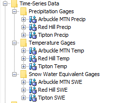
Figure 6. Precipitation, temperature, and snow water equivalent gages.
Task 4: Create a Basin Model that has subbasin elements representing three SNOTEL gages.
For this workshop, we are using subbasin elements to represent the SNOTEL gages. The subbasin area will be set to a small value and all modeling methods for the subbasin element will be set to none. Using subbasins is required because the meteorologic model is designed to compute precipitation and snowmelt for subbasin elements. The SNOTEL gage will be referred to as subbasins within the workshop.
- Create a new Basin Model using the Basin Model Manager option found under the Components tab.
- Add the Rivers and Subbasin shapefiles, saved in the "maps" folder, as background layers. The Map Layer manager is found under the View tab. You can change the display properties for each layer by highlighting the desired layer and selecting the Draw Properties option in the Map Layer window.
- Add a new subbasin element for each of the three SNOTEL gages using the Subbasin Creation Tool found in the toolbar at the top of the program window. Name the subbasins Red Hill Gage, Arbuckle MTN Gage, and Tipton Gage to correspond with the SNOTEL names. Figure 7 shows approximate locations to place the subbasin elements, the location of the subbasin elements are not critical.
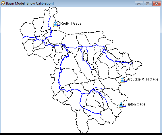
Figure 7. Basin Model with subbasin elements representing SNOTEL gages.
- Open the component editor for each of the subbasin elements and define a subbasin area of 1 square mile and choose None for Canopy, Surface, Loss, Transform, and Baseflow methods. Subbasin area is not critical as we are not focused on runoff in this workshop.
- Set the Observed SWE gage for each subbasin by selecting the Options tab on the subbasin element's component editor. Then choose the appropriate SWE gage from the drop down list. Simulated and observed SWE can be compared within HEC-HMS when linking an observed SWE gage to a subbasin element.
- Make sure that the Unit System is set to U.S. Customary and the Replace Missing option is set to Yes.
Task 5: Create a Meteorologic Model and parameterize the precipitation and snowmelt components.
- Create a Meteorologic Model named Snow Calibration, the units should be set to U.S. Customary.
- Choose the Specified Hyetograph precipitation method, Temperature Index should be selected for Snowmelt, and choose the Set to Default option for Replace Missing.
- Link the meteorologic model to the basin model created in Step D above (go to the Basins tab and choose Yes to include subbasins from the basin model).
- Expand the meteorologic model in the watershed explorer and select the Specified Hyetograph node, as shown in Figure 8. In the Specified Hyetograph component editor, select the appropriate precipitation gage for each of the three subbasins.
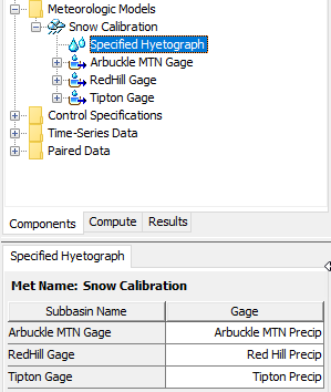
Figure 8. The Specified Hyetograph component editor with precipitation gages selected for each subbasin.
- Add the ATI-Meltrate and ATI-Coldrate paired data to the project using the Paired Data Manager under the Components tab. HEC-HMS 4.4 allows you to define a separate meltrate and coldrate function for each subbasin; however, create only one curve that will be selected by all three subbasins initially. You can create separate paired data curves for each subbasin if needed during calibration. Enter the values in Table 1 for the ATI-Meltrate curve and the values in Table 2 for the ATI-Coldrate curve.
Table 1. ATI-Meltrate function.
ATI (DegF-Day) | Meltrate (IN/DegF-Day) |
|---|---|
0 | 0.04 |
100 | 0.08 |
500 | 0.12 |
Table 2. ATI-Coldrate function.
ATI (DegF-Day) | Coldrate (IN/DegF-Day) |
|---|---|
0 | 0.02 |
500 | 0.03 |
1000 | 0.03 |
- The next step is to enter temperature index boundary condition information and parameters for each subbasin. Click on one of the subbasin nodes (within the meteorologic model portion of the watershed explorer) to open the Atmospheric Variables component editor as shown in Figure 9. Select the appropriate temperature gage for the subbasin. Then, select the Temperature Index node, below the subbasin node, to open the component editor shown in Figure 10. Enter a lapse rate of 0 DEG F / 1000 FT, a lapse rate is not required since the temperature and SWE measurements were made at the same gage site. Enter the temperature index parameters using values in Table 3. Repeat this step for the other two subbasins.
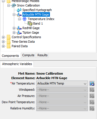
Figure 9. Atmospheric Variables component editor for a subbasin element.
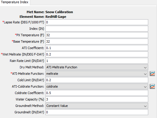
Figure 10. Temperature Index component editor for a subbasin element.
Table 3. Temperature Index initial snow model parameters.
Parameter | Value |
PX Temp (Deg F) | 32 |
Base Temp (Deg F) | 32 |
ATI-Meltrate Coefficient | 0.1 |
Wet Melt Rate | 0.20 |
Rain Rate Limit (IN/Day) | 1 |
Dry Melt Method | ATIMR Function |
ATI-Meltrate Function | Use your ATIMR function |
Cold Limit (IN/Day) | 0.2 |
ATI-Coldrate Function | Use your ATICC function |
ATI-Coldrate Coefficient | 0.5 |
Water Capacity (%) | 3.0 |
Groundmelt Constant (in/day) | 0 |
- An elevation band must be added to each of the subbasins. Right click on the subbasin's Temperature Index node in the watershed explorer. A pop-up menu should open, click the option to add an elevation band. Open the elevation band's component editor by clicking on Band 1 in the watershed explorer. With a single elevation band per subbasin, you need to set the Percent (%) parameter to a value of 100. Many of the initial snow model parameters required will be set to zero because the simulation will start at the beginning of the snow season, when there is no snowpack established. The elevation for the band is the same elevation defined for the temperature gage, 5000 ft. Table 4 contains the information to enter for elevation Band 1. Create an elevation band for all three subbasins and enter the information in Table 4.
Table 4. Initial snow conditions for elevation Band 1, assuming no initial snowpack.
Parameter | Value |
Percent (%) | 100 |
Elevation (FT) | 5000 |
Initial SWE (IN) | 0 |
Initial Cold Content (IN) | 0 |
Initial Liquid Water (IN) | 0 |
Initial Cold Content ATI (F) | 32 |
Initial Melt ATI (DegF-Day) | 0 |
Task 6: Create a simulation for the 1997 and 1998 water years and evaluate results.
- Create a Control Specifications named Snow Time Window with a start date of 02Oct1996 at time 00:00 and an end date of 01Oct1998 at time 00:00. Set the Time Interval to 1 Day (the SNOTEL data is at a 1-Day time step).
- Create a simulation run named SWE Calibration that combines the basin model, meteorologic model, and control specifications.
- Run the simulation. The simulation should take about two seconds to complete.
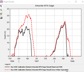
- Computed and observe SWE results can be accessed from the Results tab of the watershed explorer. Expand the watershed explorer for the Red Hill subbasin. Select the Snow Water Equivalent result first, hold down the control key and then select the Observed SWE result second. Then click the View Graph button to open a larger plot of the results. Figure 11 shows the results at the Red Hill gage using the parameters defined above. Figure 12 shows the summary table with metrics describing how well/poor the model performed.
Results for the Red Hill Gage should look similar to the other subbasins, the simulated results show that the rate of melt is slower than the observed melt rate in the spring-summer time frame. The magnitude of peak SWE is close between the observed and simulated time-series. 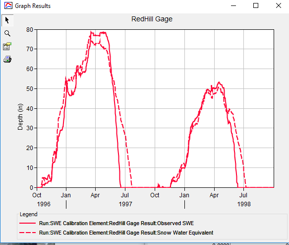
Figure 11. Modeled and observed SWE for the Red Hill gage. 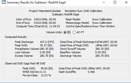
Figure 12. Summary table for the Red Hill gage.
Question 1: What can you tell from the observed vs. computed SWE plots and summary tables for all three gages/subbasins and how would you use this information to approach improving your model results?
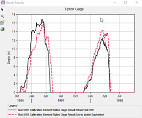
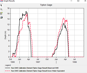
Modeled and observed SWE for the SNOTEL sites
Using the initial parameterization, the timing of when the snowpack completely disappears is delayed in the model results. There are a few factors that could contribute to this. Cold content and liquid water content both act to delay the onset of melt, though typically the impact is small. The most likely factor contributing to the delay in melt is the dry meltrate. Increasing the dry meltrate values, especially at the lower end (lower ATI values) was found to give much better results.
Task 7: Adjust the Temperature Index parameters to improve the model results.
Revisit the parameters you defined in the temperature index model. Modify the following parameters in a systematic way. Understand how the model parameter impacts the computed snow accumulation and melt, rate of melt and timing are important. Re-compute your simulation and evaluate observed vs modeled SWE to refine the model and identify parameters that provide satisfactory results for all three gages. Open computed and observed SWE results in separate plots and tables for all three subbasins. Watch the results update each time the simulation finishes. You can also add other time-series to the plots, Air Temperature and Precipitation are helpful.
- The first parameter to adjust is the ATI-Meltrate function. If you plot the Melt Rate ATI output time-series, you will see the computed result does not go beyond 40 Deg F – Day. More definition is needed in the ATI-Meltrate curve at the lower end. Also, the model needs to melt snow faster to match the melt observed in May-June. Add a row to the ATI-Meltrate table at 10 DEG F – DAY and enter a meltrate in the range of 0.06-0.10 IN/DEG F-DAY. Also, increase the meltrate at 100 DEG F-DAY to 0.15 IN/DEG F-DAY. After running the simulation, you should notice an improvement in model results with the increased meltrates. Try adjusting the meltrate to match the timing when the snowpack disappears. You can create a separate meltrate curve for each subbasin if needed.
- Next, try modifying the ATI-Coldrate curve to see how this parameter impacts the model. Larger values will delay melt (adds more energy to freeze liquid water), smaller values will result in earlier melt.
- Modify the PX temperature. A larger value will increase the snowpack during the winter (more precipitation is determined to be frozen and not liquid).
- Modify the Wet Meltrate. The wet meltrate is only applied during those time steps when rain on snow occurs, and the precipitation rate exceeds the rain rate limit.
Make note of your NSE score for each of the SnoTel gages. The team with the highest NSE score per gage will be awarded a prize. Other metrics that are important with SWE are date of peak SWE and date when the SWE melts off.
Question 2: What is your final parameter set per subbasin/gage? Which parameters were more influential for simulating SWE and matching observations?
Besides the ATI-Meltrate, another sensitive parameter was the PX temperature. The PX temperature was increased to 33 degrees F for the Red Hill and Tipton SNOTEL gages. The increase in the PX temperature resulted in more accumulation of snow during the season. The ATI-Coldrate paired data curve was modified to reduce the amount of delay in melt when temperature goes above the Base Temperature and when melt begins.
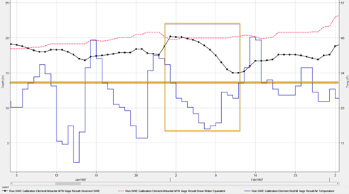
Question 3: Create a plot for the Arbuckle MTN gage that includes Computed SWE, Observed SWE, and Temperature. Zoom into the time frame between January 20 and February 15 - 1997. Do the observed SWE and Temperature datasets seem reasonable in this time frame?
The following figure shows the Observed Temperature and SWE for January 1997, look inside the rectangle. Notice that the observed SWE decreases from 20 inches to 15 inches even though the temperature is below freezing. There could be other processes that are impacting the snowpack, like sublimation. The HEC-HMS model will not be able to track the trend in observed SWE during this period if other processing not included in HEC-HMS are impacting the snowpack. Another possibility are errors in the gage measurements.
Question 4: Describe some of the limitations when using daily accumulated precipitation and averaged temperature data as boundary conditions.
Daily data does not include the diurnal pattern in temperature, when temperatures are colder at night and warmer during the day. Cold temperatures at night can add cold content to the snowpack that offsets some melt during the day. Using daily average temperature does not capture the diurnal temperature pattern, the model will not simulate the increase/decrease in cold content due to the diurnal pattern in temperature. Precipitation can be dynamic within an event. A storm can start out warmer, with mostly liquid precipitation. Then, the temperature can drop as a cold front passes, and liquid precipitation turns into snow. Using daily accumulated precipitation with a daily average temperature might not capture the dynamic nature of rain/snow during some storm events.
Final project files: MainstemColumbia.zip