Download PDF
Download page Computing a PMF/Statistical Event Simulation and Analyzing Results.
Computing a PMF/Statistical Event Simulation and Analyzing Results
The goal of this workshop is to become familiar with output from the Temperature Index model. The Elevation Band Temperature Index snowmelt method will be used to simulate accumulation and melt of snow during a hypothetical flood event. The hypothetical event is a short duration rain on snow type of event. The wet meltrate parameter will be adjusted to match total event snowmelt as computed externally to HEC-HMS.
HEC-HMS version 4.9 was used to create this workshop.
Download the Initial Project Files here - Interbay_Dam_Initial.zip
The workshop example uses the watershed upstream of Interbay Dam, located in the Sierra Nevada mountains in California. The elevation range is 2,500 feet to 9,000 feet and the average elevation in the watershed is 5,900 feet. The watershed also includes LL Anderson Dam (forms the French Meadows Reservoir). This workshop picks up where the Creating a Temperature Index Snowmelt Model for a PMF/Statistical Event Simulation workshop finished.
Major tasks in this workshop include:
- Run a Simulation and Determine the Amount of Snowmelt
- Find other Snowmelt Model Results in Output DSS File
- Refine the Wet Meltrate
- Set up an Alternative Simulation with no Snowmelt
- Compare Model Results between Simulation Alternatives
Run a Simulation and Determine the Amount of Snowmelt
The StatisticalStorm simulation combines the CalibratedModel basin model, the StatisticalStorm meteorologic model, and the StatisticalStorm control specifications. In this step, we will look at Temperature Index results available from HEC-HMS.
- Run the StatisticalStorm simulation.
- Go to the Results tab in the Watershed Explorer, expand the tree for the StatisticalStorm simulation run, and expand the tree for the MF_American_Rv_S30 subbasin element. Notice the time-series results available for the subbasin element, shown below.
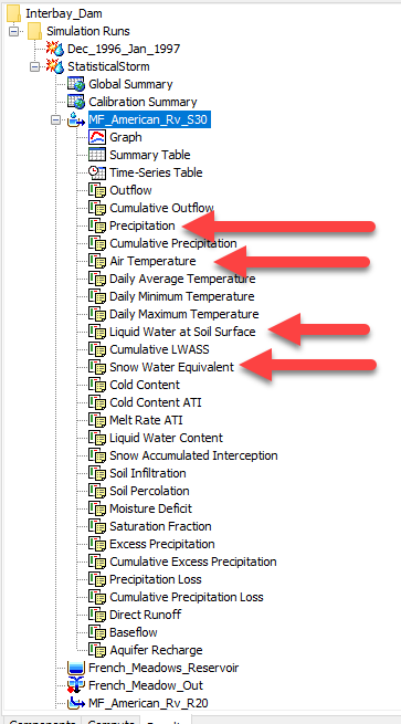
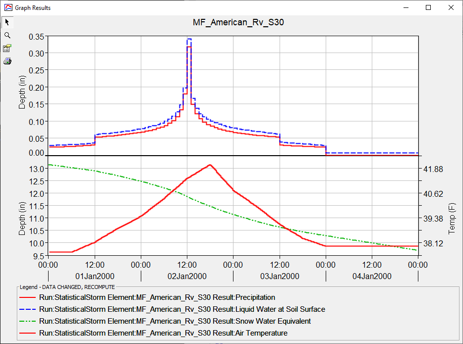
Hold down the control key and select the Precipitation, Air Temperature, Liquid Water at Soil Surface (LWASS), and Snow Water Equivalent (SWE) results. Click the View Graph button to open a plot like the one below (you will have to edit the line properties to make your results resemble those below). Notice the LWASS results are always greater than the precipitation time-series, which means the snowpack is melting and contributing to available water on top of the land surface. The SWE decreases throughout the event and the basin average temperature is above 32 degrees F for the entire event.

SWE Results
The computed SWE represents the basin average SWE. Elevation bands higher than 6,000 ft had an initial SWE of 20 inches (SWE is typically not limiting for the extreme floods that occur in the winter months, 20 inches was used to insure snowmelt throughout the event for elevations above 6,000 ft. The basin average initial SWE is slightly above 13 inches.
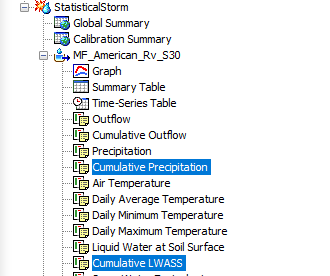
- Hold down the control key and select Cumulative Precipitation and Cumulative LWASS. You should notice the results are plotted in the preview plot located in the lower left.
- Click the View Time Series Table button to open a time-series table.
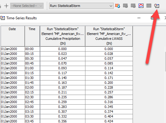
- Scroll to the bottom of the time-series results table and you will see the cumulative precipitation is 18.10 inches and the cumulative LWASS is 21.54 inches. If the cumulative LWASS is less than the precipitation then that means some of the precipitation fell as snow and was added to the snowpack. If the LWASS is greater than the precipitation, then that means some of the snowpack melted during the simulation. Results show that 3.44 inches (cumulative LWASS - cumulative precipitation) of the SWE held in the snowpack melted and contributed to precipitation to generate the LWASS time-series.
Find other Snowmelt Model Results in the Output DSS File
Another interesting way to evaluate results from an elevation band Temperature Index model is to look at results for each elevation band. You cannot access elevation band information from the HEC-HMS interface, but you can access these results from output DSS files.
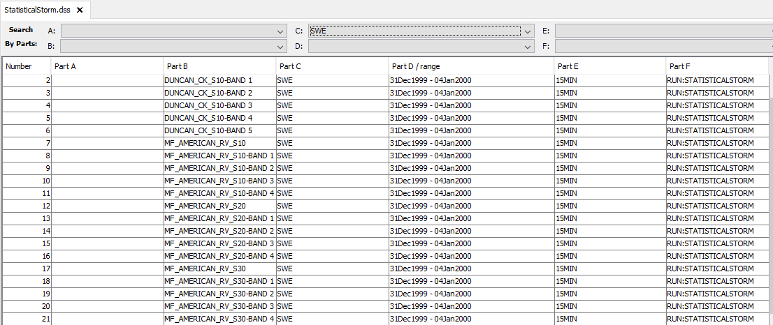
- Open HEC-DSSVue and open the StatisticalStorm.dss file and plot SWE results for each elevation band in the MF_American_Rv_S30 subbasin.
- As shown below, change the C part pathname to SWE. You should see 21 records that include basin average SWE and SWE computed for each elevation band.
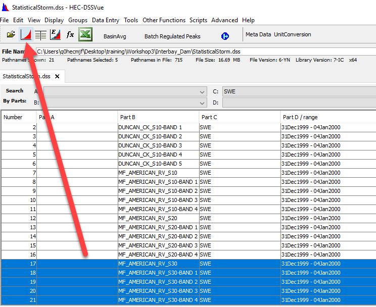
- Select all records for the MF_AMERICAN_RV_S30 subbasin and click the Plot button.
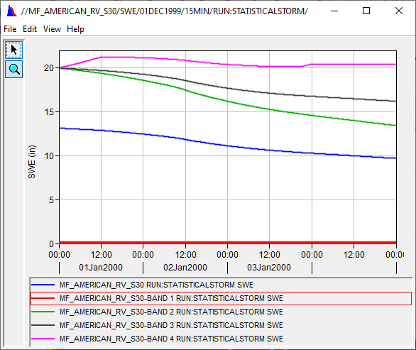
- As shown below, the lowest elevation band (5,000 feet to 6,000 feet) had no snowpack. The highest elevation band (8,000 feet to 9,000 feet) saw the SWE increase during the first 12 hours of the simulation (because the air temperature was less than the PX and Base temperatures). The area weighted average SWE, the blue line, is the value computed within HEC-HMS. Notice the SWE decreases the most for elevation band 2 because this elevation band had the highest temperature among elevation bands 2, 3, and 4.
Refine the Wet Meltrate
The Wet Meltrate can be the most impactful parameter when modeling rain on snow conditions like those represented in the StatisticalStorm simulation. As shown in previous steps, the 3-day precipitation total is over 18 inches and the temperature sequence is above freezing for most of the watershed used in this workshop. One way to determine a reasonable Wet Meltrate for hypothetical storms is to compute the total snowmelt using energy balance derived equations and iteratively setting the Wet Meltrate until the simulated snowmelt matches the snowmelt from the energy balance equations.
Engineering Manual (EM) 1110-2-1406 includes Equations 5-19 & 5-20 which are energy balanced equations for estimating daily snowmelt in heavily or partially forested areas. These equations require temperature, windspeed, and precipitation. Guidance in reference manuals can be used to estimate both the temperature and windspeed time-series for extreme events. For example, there is a procedure defined in Hydrometeorological Report Number 58 (HMR 58) for California that shows how to estimate temperature, windspeed and other meteorologic variables for the Probable Maximum Precipitation event.
Using the energy balance equations and the procedure for estimating meteorologic data during a PMP, the total event snowmelt for the watershed upstream of LL Anderson Dam (MF_American_Rv_30) was estimated to be 3.4 inches and the total event snowmelt for the area between Interbay Dam and LL Anderson Dam was estimated to be 2.0 inches. The MF_American_Rv_20 and MF_AMerican_Rv_S10 subbasins have most of their terrain below 6,000 feet. Only the Duncan_Ck_S10 subbasin has a considerable amount of its terrain above 6,000 feet.
As shown in the first task, you can compare the difference in the cumulative precipitation and cumulative LWASS time-series to compute the simulated amount of snowmelt. We saw the computed amount of snowmelt was 3.44 inches for the MF_American_Rv_30 subbasin.
- Check the amount of snowmelt from the Duncan_Ck_S10 subbasin. You should see the cumulative precipitation is 18.10 inches and the cumulative LWASS is 20.68 inches, which results in 2.58 inches of snowmelt.
- As mentioned above, the energy balance equation estimated 3.4 inches of snowmelt for the MF_American_Rv_S30 subbasin and 2.0 inches of snowmelt for the Duncan_Ck_S10 subbasin. No adjustment to the Wet Meltrate is needed for the MF_American_Rv_S30 subbasin. The Wet Meltrate needs to be reduced for the Duncan_Ck_S10 subbasin in order to reduce the amount of snowmelt.
- Leave the time-series table containing cumulative precipitation and cumulative LWASS results open for the Duncan_Ck_S10 subbasin. HEC-HMS will automatically update the results in the time-series table each time the simulation is computed.
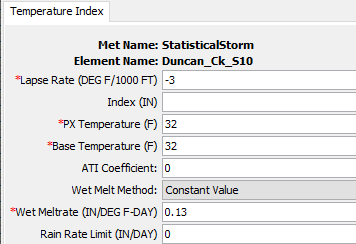
- Open the Temperature Index component editor for the Duncan_Ck_S10 subbasin. Adjust the Wet Meltrate, change it to 0.18 In/Deg F-Day and rerun the StatisticalStorm simulation. You should notice the cumulative LWASS decreased to 20.51 inches, which means the total snowmelt was 2.41 inches.
- The target total event cumulative LWASS is 20.1 inches (which means 2.0 inches of SWE melted during the simulation). Continue decreasing the wet meltrate until the target amount of snowmelt is computed. A Wet Meltrate of 0.13 In/Deg F-Day was found to reproduce the desired amount of snowmelt.
Set up an Alternative Simulation with no Snowmelt
The following steps show how to set up an alternative simulation that contains no snowmelt. A similar procedure could be followed to perform a sensitivity analysis and evaluate changes to results caused by varying wet meltrates.
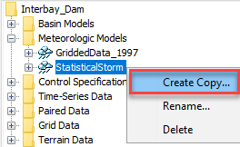
- To create a copy of the StatisticalStorm meteorologic model, select the name in the tree, click the right mouse button, and choose Create Copy.
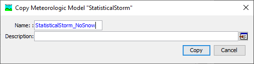
- Name the new meteorologic model StatisticalStorm_NoSnow and click the Copy button.
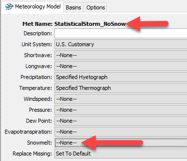
- Open the Component Editor for the StatisticalStorm_NoSnow meteorologic model and set the Snowmelt method to None.
- Go to the Compute tab in the Watershed Explorer and expand the Simulation Run folder. Select the StatisticalStorm simulation and click the right mouse button. Choose the Create Copy menu option.
- Enter a new simulation run name of StatisticalStorm_NoSnow.
- Open the Component Editor for the new simulation and change the Meteorologic Model to StatisticalStorm_NoSnow as shown below.
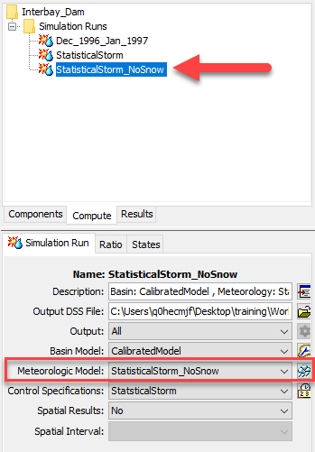
- Run the StatisticalStorm_NoSnow simulation and check results on the Results tab for one of the subbasin elements. No snowmelt results should be visible.
Compare Model Results between Simulation Alternatives
It is easy to compare results at different elements within a simulation or between simulations. The key is to access results from the Results tab of the Watershed Explorer.
- Go to the Result tab in the Watershed Explorer and expand the tree for both the StatisticalStorm and StatisticalStorm_NoSnow simulations.
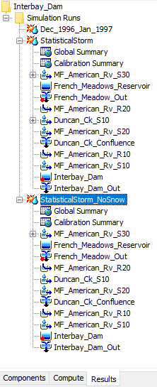
- Select the MF_American_Rv_S30 subbasin element to expand the tree within both simulations. Hold down the control key and select the Outflow time-series from both simulations.
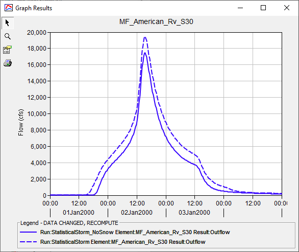
- Click the View Graph button to open a plot of both Outflow results. You can edit the plot draw properties if needed. As shown below, the simulation that included snowmelt generated more runoff and a higher peak flow than the simulation that did not include snowmelt. You can also click the View Time-Series Table button when results are selected to see a table with values for each time-step.
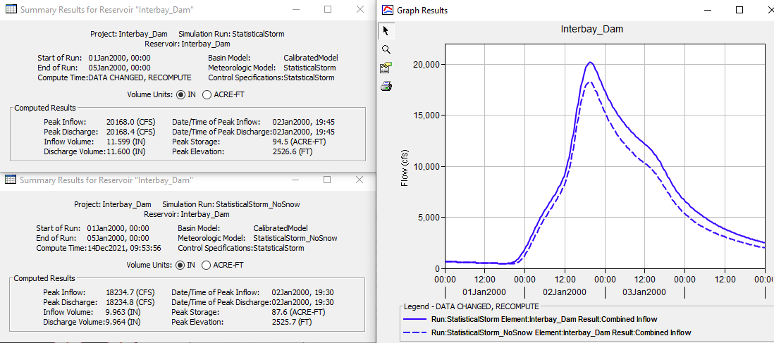
- You can open the element summary tables to view information as shown below. The element summary tables show differences in peak flow and discharge volume. The summary table is the second node beneath each element name on the Results tab.
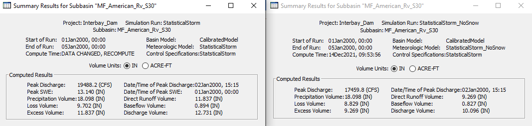
- As you can see in the figure below, including snowmelt in the simulation caused the peak inflow into Interbay Dam to increase from 18,235 cfs to 20,168 cfs. You can also see the difference in peak reservoir storage and elevation as well (included in the summary tables and also time-series results).