Download PDF
Download page Creating a Temperature Index Snowmelt Model for a PMF/Statistical Event Simulation.
Creating a Temperature Index Snowmelt Model for a PMF/Statistical Event Simulation
The goal of this workshop is to configure a meteorologic model to use time-series precipitation and temperature to simulate a hypothetical event in HEC-HMS. The Elevation Band Temperature Index snowmelt method will be used to simulate accumulation and melt of snow during the hypothetical flood event. The hypothetical event is a short duration rain on snow type of event.
HEC-HMS version 4.9 was used to create this workshop.
Download the Initial Project Files here - Interbay_Dam_Initial.zip
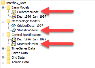
The workshop example uses the watershed upstream of Interbay Dam, located in the Sierra Nevada mountains in California. The elevation range is 2,500 feet to 9,000 feet and the average elevation in the watershed is 5,900 feet. The watershed also includes LL Anderson Dam (forms the French Meadows Reservoir). This workshop picks up where the Creating a Temperature Index Snowmelt Model for a Historical Event Simulation workshop finished. As shown in the figure below, the CalibratedModel basin model and StatisticalStorm meteorologic model and control specifications have been added to the project for you. Since the PMP and statistical storms use precipitation and temperature time-series data, we will have to configure an elevation band Temperature Index model.
Major tasks in this workshop include:
- Enter PMP/Statistical Event Precipitation Data
- Enter PMP/Statistical Event Temperature Data
- Define Elevation Bands
- Complete Data Requirements for the Temperature Index Snowmelt Model
Enter PMP/Statistical Event Precipitation Data
The following table contains the precipitation data for the hypothetical storm (we will assume uniform precipitation for all four subbasins in the HEC-HMS project). The event lasts three days and there are precipitation totals for each hour. A precipitation time-series gage needs to be added to the Interbay Dam HEC-HMS project.
Time (hours) | Incremental Precipitation (inches) | Cumulative Precipitation (inches) | Time (hours) | Incremental Precipitation (inches) | Cumulative Precipitation (inches) | Time (hours) | Incremental Precipitation (inches) | Cumulative Precipitation (inches) |
|---|---|---|---|---|---|---|---|---|
| 1 | 0.093 | 0.093 | 25 | 0.271 | 4.32 | 49 | 0.267 | 14.275 |
| 2 | 0.094 | 0.187 | 26 | 0.28 | 4.599 | 50 | 0.259 | 14.535 |
| 3 | 0.096 | 0.283 | 27 | 0.289 | 4.889 | 51 | 0.253 | 14.788 |
| 4 | 0.098 | 0.381 | 28 | 0.301 | 5.189 | 52 | 0.247 | 15.035 |
| 5 | 0.1 | 0.48 | 29 | 0.314 | 5.503 | 53 | 0.241 | 15.276 |
| 6 | 0.102 | 0.582 | 30 | 0.329 | 5.832 | 54 | 0.236 | 15.512 |
| 7 | 0.104 | 0.686 | 31 | 0.348 | 6.181 | 55 | 0.232 | 15.744 |
| 8 | 0.106 | 0.793 | 32 | 0.373 | 6.553 | 56 | 0.227 | 15.971 |
| 9 | 0.109 | 0.901 | 33 | 0.405 | 6.959 | 57 | 0.223 | 16.195 |
| 10 | 0.111 | 1.012 | 34 | 0.452 | 7.411 | 58 | 0.22 | 16.414 |
| 11 | 0.114 | 1.126 | 35 | 0.53 | 7.941 | 59 | 0.216 | 16.631 |
| 12 | 0.117 | 1.243 | 36 | 0.72 | 8.661 | 60 | 0.213 | 16.843 |
| 13 | 0.211 | 1.454 | 37 | 1.27 | 9.931 | 61 | 0.118 | 16.962 |
| 14 | 0.214 | 1.669 | 38 | 0.598 | 10.529 | 62 | 0.115 | 17.077 |
| 15 | 0.218 | 1.887 | 39 | 0.485 | 11.014 | 63 | 0.113 | 17.19 |
| 16 | 0.221 | 2.108 | 40 | 0.426 | 11.441 | 64 | 0.11 | 17.3 |
| 17 | 0.225 | 2.333 | 41 | 0.388 | 11.828 | 65 | 0.107 | 17.407 |
| 18 | 0.23 | 2.563 | 42 | 0.36 | 12.188 | 66 | 0.105 | 17.512 |
| 19 | 0.234 | 2.797 | 43 | 0.338 | 12.526 | 67 | 0.103 | 17.615 |
| 20 | 0.239 | 3.036 | 44 | 0.321 | 12.848 | 68 | 0.101 | 17.716 |
| 21 | 0.244 | 3.28 | 45 | 0.307 | 13.155 | 69 | 0.099 | 17.815 |
| 22 | 0.25 | 3.53 | 46 | 0.295 | 13.449 | 70 | 0.097 | 17.911 |
| 23 | 0.256 | 3.786 | 47 | 0.284 | 13.734 | 71 | 0.095 | 18.007 |
| 24 | 0.263 | 4.049 | 48 | 0.275 | 14.009 | 72 | 0.093 | 18.1 |
- Select the Components | Time-Series Data Manager option.
- Make sure the Data Type is set to Precipitation Gages and Click the New button.
- Name the Precipitation Gage StatisticalStormPrecip and click the Create button.

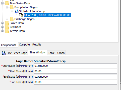
- Expand the Time-Series Data node in the Watershed Explorer. Then expand the Precipitation Gages node and the StatisticalStormPrecip gage node as shown below. Click the Time Window node to open the Time Window tab within the Watershed Explorer.
- The Control Specifications for the StatisticalStorm simulation was set to 01Jan2000 at 00:00 through 05Jan2000 at 00:00. Change the End Date for the precipitation gage to 05Jan2000.
- Select the Time-Series Gage tab and make sure the precipitation gage Units are set to Incremental Inches and the Time Interval is set to 1 Hour.
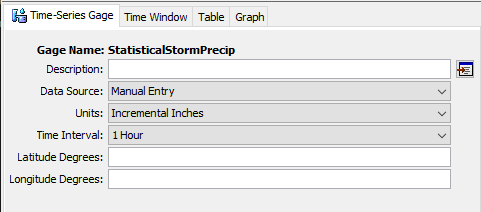
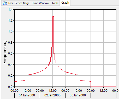
- Select the Table tab and copy/paste the incremental precipitation as contained in the table above into the HEC-HMS table (copy and paste the information in the table above into Excel first, then copy and paste just the precipitation values into the HEC-HMS table). Be sure to enter 0 inches of precipitation from 04Jan2000, 01:00 through 05Jan2000, 00:00. Enter zero in the first blank cell, highlight this cell and the remaining empty cells, right click somewhere in the highlighted fields, and select fill. Select “Repeat first value,” and select OK.
- Select the Graph tab, the precipitation hyetograph should be similar to the figure below.
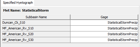
- Now that the precipitation gage has been added to the project, it needs to be selected in the StatisticalStorm meteorologic model. Select the Specified Hyetograph node in the StatisticalStorm Meteorologic Model to open the Component Editor.
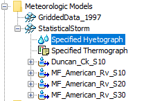
- Select the StatisticalStormPrecip gage for each subbasin element as shown below.
Enter PMP/Statistical Event Temperature Data
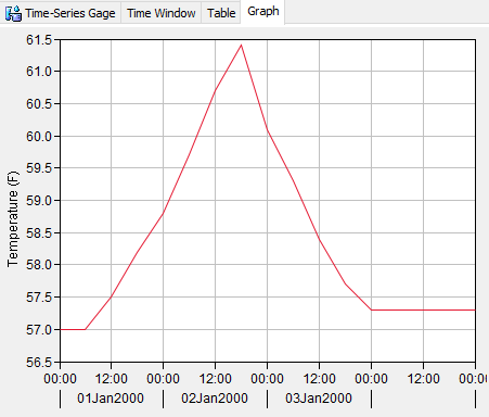
The following table contains the temperature data for the hypothetical storm. The event lasts three days and there are instantaneous temperature values at six hour increments. A temperature time-series gage needs to be added to the Interbay Dam HEC-HMS project.
Time (hours) | Instantaneous Temperature (Deg F) |
|---|---|
| 0 | 57.0 |
| 6 | 57.0 |
| 12 | 57.5 |
| 18 | 58.2 |
| 24 | 58.8 |
| 30 | 59.7 |
| 36 | 60.7 |
| 42 | 61.4 |
| 48 | 60.1 |
| 54 | 59.3 |
| 60 | 58.4 |
| 66 | 57.7 |
| 72 | 57.3 |
- Select the Components | Time-Series Data Manager option.
- Make sure the Data Type is set to Temperature Gages and click the New button.
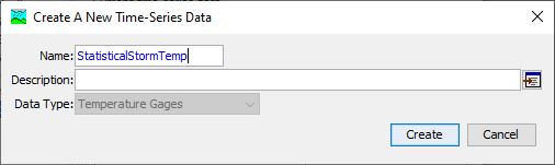
- Name the Temperature Gage StatisticalStormTemp and click the Create button.
- Expand the Time-Series Data node in the Watershed Explorer. Then expand the Temperature Gages node and the StatisticalStormTemp gage node as shown below. Click the Time Window node to open the Time Window tab within the Watershed Explorer.
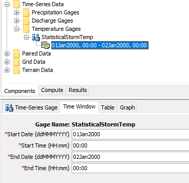
- The Control Specifications for the StatisticalStorm simulation was set to 01Jan2000 at 00:00 through 05Jan2000 at 00:00. Change the End Date for the temperature gage to 05Jan2000.
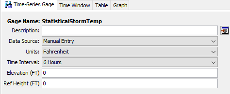
- Select the Time-Series Gage tab and make sure the temperature gage Units are set to Fahrenheit and the Time Interval is set to 6 Hours. Set the Elevation and Ref Height to 0 Feet.
- Select the Table tab and enter the temperature data contained in the table above into the HEC-HMS table. Be sure to enter 57.3 Degrees F from 04Jan2000, 06:00 through 05Jan2000, 00:00. Enter 57.3 Degrees F in the first blank cell, highlight this cell and the remaining empty cells, right click somewhere in the highlighted fields, and select fill. Select “Repeat first value,” and select OK.
- Select the Graph tab, the temperature plot should be similar to the figure below.
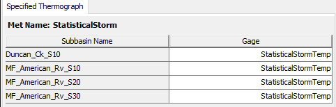
- Now that the temperature gage has been added to the project, it needs to be selected in the StatisticalStorm Meteorologic Model. Select the Specified Thermograph node in the StatisticalStorm Meteorologic Model to open the Component Editor.
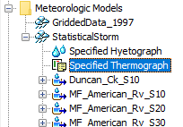
- Select the StatisticalStormTemp gage for each subbasin element as shown below.
Define Elevation Bands
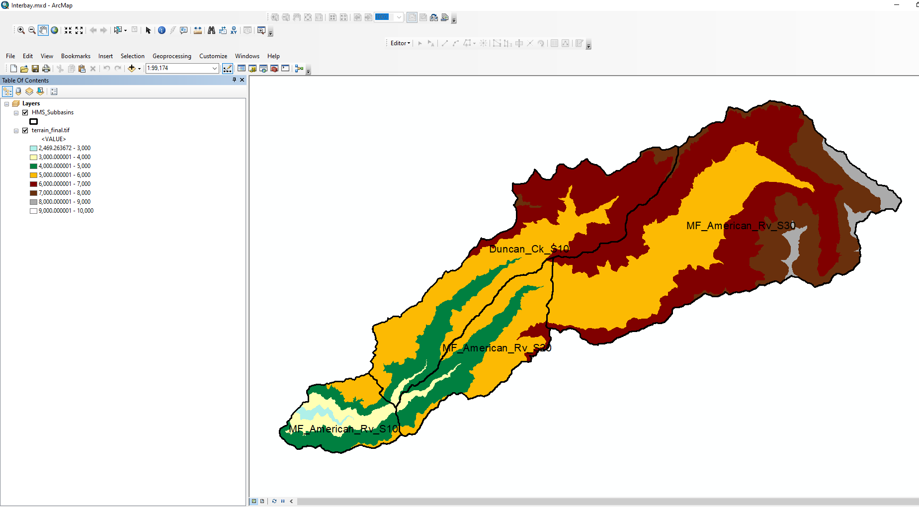
HEC-HMS requires the modeler define the percentage of the subbasin area within each elevation band. ArcGIS can be used to compute this information for you. An ArcGIS project is located in the ...\\GIS directory. Double click the Interbay.mxd file to open the ArcGIS project. (The ArcMap project was created with ArcGIS 10.4. If you have an older version, then you will not be able to open the project. Instead, use the version of ArcGIS on your computer and load the terrain and subbasin shapefile into a ArcMap project. Then edit the terrain data's legend to match what is shown in the figure below.) You should see two GIS layers already added to the project. The symbology for the terrain data has been edited using the Classified option, and elevation ranges were defined to correspond to elevation bands at 1,000 foot intervals.
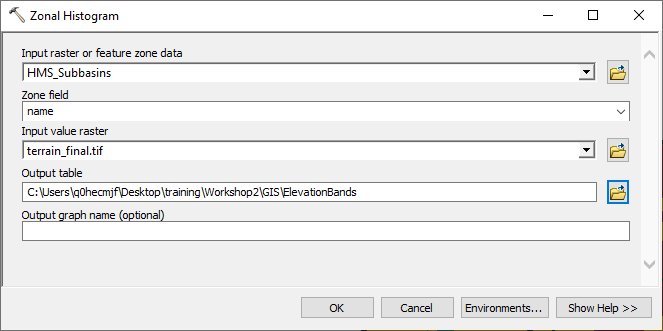
- Open the Zonal Histogram tool (you can find this tool in the Search bar).
- Select the HMS_Subbasins layer as the Zone data.
- The name attribute should be selected as the Zone field. The name attribute contains the subbasins names as defined in the HEC-HMS model.
- Select the terrain_final.tif layer as the input Raster.
- Choose a location and enter a name for the results table. The complete Zonal Histogram editor is shown below. Press the OK button to run the tool.
- Open the summary table created by the Zonal Histogram tool. As shown below, the tool counts the number of elevation grid cells that are within each elevation range.
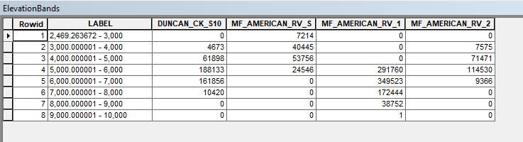
- Export the summary table as a *.txt file and open it within Excel. Use the Delimited option in Excel to separate the data into the appropriate columns. You might need to edit the column widths to see the column headers. There is a character limit in ArcGIS, the MF_American_RV subbasin names were shortened. MF_AMERICAN_RV_S30 should be the subbasin with the highest elevations. MF_AMERICAN_RV_S10 should be the subbasin with the lowest elevations.
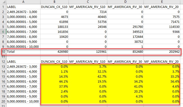
- Edit the Excel page to sum the total number of grid cells within each subbasin and then compute the area percentage for each elevation range, as shown in the figure below.
Complete Data Requirements for the Temperature Index Snowmelt Model
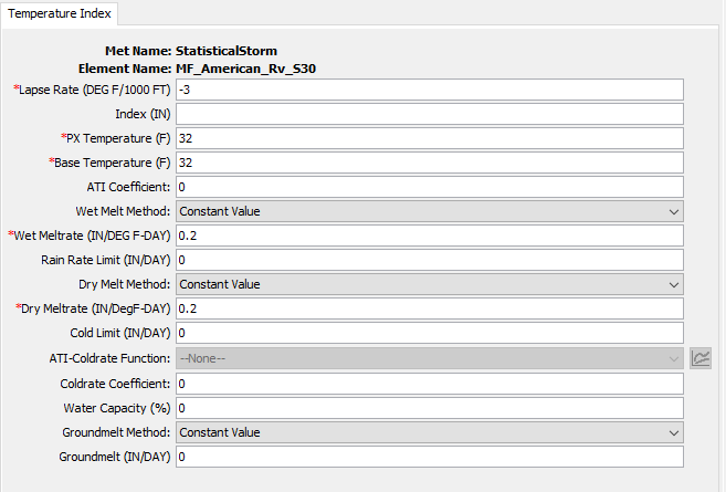
The figure below shows the Temperature Index Component Editor for the MF_American_Rv_S30 subbasin. The same parameter values were duplicated for the other three subbasins. These are generic parameter values and should be refined with local knowledge or additional information. The main parameters for a rain on snow event simulation are the PX Temperature, Base Temperature, and Wet Meltrate parameters. The Computing a PMF/Statistical Event Simulation and Analyzing Results workshop shows how to set the Wet Meltrate using computed snowmelt from an energy balance equation. The remaining items needed to finish the StatisticalStorm meteorologic model in order for the simulation to run are to create elevation bands for each subbasin element and populate each elevation band with area percentages and initial conditions.
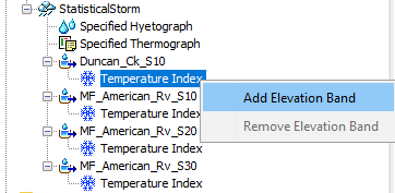
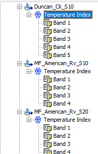
- Expand the Watershed Explorer so you can see the Temperature Index node beneath each subbasin element. To add an elevation band, select the Temperature Index node and click the right mouse button. Select the Add Elevation Band menu option as shown below.
Add 5 elevation bands to the Duncan_Ck_S10 subbasin, 4 elevation bands to the MF_American_Rv_S30 subbasin, 4 elevation bands to the MF_American_Rv_S20 subbasin, and 4 elevation bands to the MF_American_Rv_S10 subbasin.
The following table contains the final area percentages for each elevation band within a subbasin. The values were slightly modified from those computed above so that the total area percent is exactly 100%. HEC-HMS will stop a simulation if the area percentages do not sum to exactly 100%.
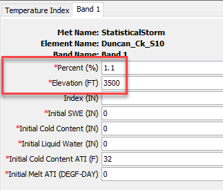
Elevation Range Duncan_Ck_S10 MF_American_Rv_S30 MF_American_Rv_S20 MF_American_Rv_S10 2,000 - 3,000 0.0% 0.0% 0.0% 5.7% 3,000 - 4,000 1.1% 0.0% 3.8% 32.1% 4,000 - 5,000 14.5% 0.0% 35.2% 42.7% 5,000 - 6,000 44.1% 34.3% 56.4% 19.5% 6,000 - 7,000 37.9% 41.0% 4.6% 0.0% 7,000 - 8,000 2.4% 20.2% 0.0% 0.0% 8,000 - 9,000 0.0% 4.5% 0.0% 0.0% 9,000 - 10,000 0.0% 0.0% 0.0% 0.0% - Starting with the Duncan_Ck_S10 subbasin, enter the area percentage for each elevation band. As shown in the figure below, use the midpoint of each elevation band to represent the Elevation for the band. For example, the Elevation should be set to 3500 feet for the elevation band representing the subbasin area located between 3,000 feet and 4,000 feet.
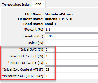
Within the Component Editor for each elevation band, set all initial condition variables to default values. Set Initial Cold Content to 0 inches, Initial Liquid Water to 0 inches, Initial Cold Content ATI to 32 Deg F, and Initial Melt ATI to 0 Deg F-Day. The Initial SWE will be assumed 0 inches for elevation bands below 6,000 feet. Use an Initial SWE of 20 inches for those elevation bands above 6000 feet.
- In the Watershed Explorer, expand the CalibratedModel basin model node. The CalibratedModel basin model was created by copying the Dec_1996_Jan_1997 basin model. Then, the transform method was changed from ModClark to Clark unit hydrograph. The elevation band Temperature Index method can not be applied to subbasins set to use the ModClark transform option. You can confirm the Clark transform method is selected by opening the component editor for each subbasin and checking the Transform method.
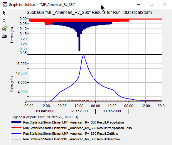
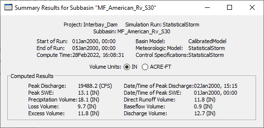
- Within the Compute toolbar, select the StatisticalStorm simulation and press the Compute button. The simulation should successfully run to completion if all meteorologic data has been defined. The following figures show the computed results for the MF_American_Rv_S30 subbasin. The following workshop will dive more into evaluating model results.