Download PDF
Download page Comparison of Post-fire Simulations with and without Dynamic Surface.
Comparison of Post-fire Simulations with and without Dynamic Surface
In this section, you will compare the results of post-fire simulations with and without the Dynamic Surface method. You will create and parameterize 3 additional Basin Models. Each of these Basin Models will use the Simple Surface method and a the Deficit and Constant Loss method to attempt to simulate the watershed's post-fire response. The minimum, average, and maximum infiltration values were used in the Deficit and Constant Loss method and are tabulated below.
| Basin Model Name | Deficit and Constant Constant Loss Rate (in/hr) |
|---|---|
| PostFire_MaxLoss | 0.5 |
| PostFire_AvgLoss | 0.3 |
| PostFire_MinLoss | 0.15 |
If time allows, follow the steps below to parameterize three additional Basin Models and compute the results. The results of the simulations are provided at the end of this page.
Post-fire Simulations with Simple Surface Method
- In the Watershed Explorer, expand the Basin Models folder.
- Right click on the PostFire_DynamicSurface basin model and select Create Copy....
- Enter PostFire_MinLossRate as the basin name and click the Copy button.
- Expand the node for the PostFire_MinLossRate basin model. Select the ArroyoSeco_S10 subbasin node.
- In the Component Editor, navigate to the Subbasin tab. Next to Surface Method, select Simple Surface from the drop-down menu, as shown in the figure below.

Navigate to the Surface tab in the Component Editor and enter an Initial Storage of 0% and a Max Storage of 0 in. These parameters are the same as those calibrated using the Dynamic Surface method in the previous task.

Selecting the Simple Surface method with an Initial Storage of 0% and a Max Storage of 0 in is equivalent to selecting --None-- as the Surface method.
- Navigate to the Loss tab in the Component Editor and enter 0.15 in/hr in the Constant Rate field.
- In the Watershed Explorer, expand the Meteorologic Models folder.
- Select the LAPW_Interp_PRISM_Bias node and navigate to the Basins tab in the Component Editor.
- Under the Include Subbasins header, select Yes from the drop-down menu to link the PostFire_MinLossRate subbasin to the LAPW_Interp_PRISM_Bias meteorologic model.
- Click the Save button.
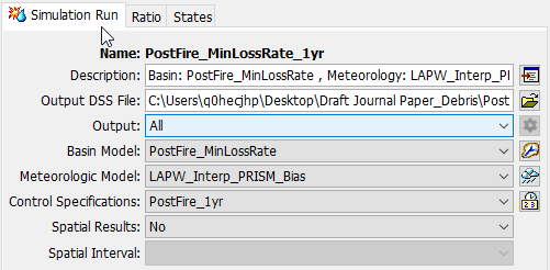
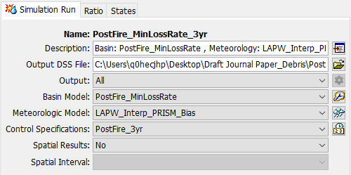
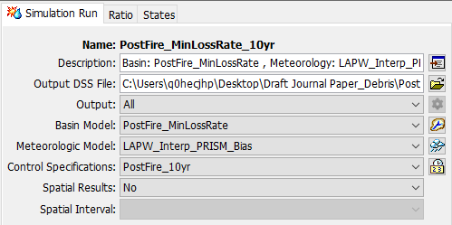
- Create 3 simulation runs named PostFire_MinLossRate_1yr, PostFire_MinLossRate_3yr, and PostFire_MinLossRate_10yr with the following components:
- Basin Model: PostFire_MinLossRate
- Meteorologic Model: LAPW_Interp_PRISM_Bias
- Control Specification: PostFire_1yr, PostFire_3yr, or PostFire_10yr
- Check that the Simulation Run selections match the figures below.
- Compute all 3 simulations and examine the results.
- Repeat the above steps to create 2 additional Basin Models, PostFire_AvgLossRate and PostFire_MaxLossRate, with Loss | Constant Rate values of 0.3 and 0.5 in/hr, respectively. For each Basin Model, create 3 additional simulations of length 1, 3, and 10 years, using the previously created Control Specifications.
Comparison of Post-fire Simulations with and without the Dynamic Surface Method
The results from the twelve simulations computed in this tutorial are shown in the figures below. Each row of figures represents a simulation method: Dynamic Surface (DS), Simple Surface with Average Loss Rate (SSAL), Simple Surface with Minimum Loss Rate (SSMnL), and Simple Surface with Maximum Loss Rate (SSMxL). Each column of figures represents a simulation period: 1, 3, and 10 years. Discussion is provided before each row of figures.
Percent Bias Computation
In HEC-HMS, the summary statistics are computed using all time steps where the observed data is defined (i.e. not missing). For example, percent bias (PBIAS) is computed as:
PBIAS (\%) = 100 \[ \sum_{i=1}^{n} \frac{S_i - O_i}{O_i} \]
where S represents the simulated values and O represents the observed values.
A positive PBIAS value indicates that the simulated discharge exceeded the observed discharge and a negative PBIAS value indicates that the observed discharge exceeded the simulated discharge.
The runoff volume, expressed as a depth, in the Summary Results Table is the sum of the discharge for all time steps in which discharge was defined. Observed discharge at the Arroyo Seco outlet is missing for some time steps. Therefore, for some simulation periods, the Summary Results Tables show negative PBIAS values but the computed volume exceeds the observed volume.
In general, model performance improves as the simulation period is reduced. This is typical of continuous simulations, since a single set of parameters is used to represent watershed conditions. The Pak and Lee Dynamic Surface method outperformed the Simple Surface and Deficit and Constant Loss method across all simulation time periods.
The Simple Surface with average Constant Loss Rate simulations produce reasonable results, particulary for the 1- and 3-year simulations. The results from the 10-year simulation, however, are poor. In the 10-year simulation, the Nash-Sutcliffe efficiency coefficient is negative, meaning that mean of the observed discharges is a better predictor than the simulated results.

Using the maximum Constant Loss Rate (0.5 in/hr) underpredicts the discharge during the 1- and 3-year simulations. In the first few years post-fire, the burnt soil's ability to infiltration water is significantly lower than unburnt soil. Therefore, using the maximum Constant Loss Rate during years 0-3 post-fire substantially overpredicts the infiltration capacity of the soil. The results of the 10-year simulation during years 3-10 are reasonable. For some of the flood events that occur in years 3-10, the maximum Constant Loss Rate results show improvement over the Dynamic Surface results.

Using the minimum Constant Loss Rate (0.15 in/hr) drastically overpredicts the discharge during all three simulation periods. While a Constant Loss Rate of 0.15 in/hr is a reasonable estimate immediately post-fire (during the January 2010 event), the use of this value in long-term post-fire simulations overpredicts the runoff.
