Download PDF
Download page Extreme Precipitation-Frequency Events.
Extreme Precipitation-Frequency Events
Workshop summary: you will use a watershed model for the watershed above Schafer Dam/Lake Success near Porterville, CA to assess the magnitude and uncertainty of extreme precipitation-frequency events routed through HEC-HMS.
Project Files
HEC-HMS Version
This workshop was developed with HEC-HMS v4.12 beta 5.
Download the initial project file: Extreme_Precip_Freq.zip
Introduction
For estimating hydrologic hazard curves for dams, an approach based on routing extreme precipitation-frequency events through a rainfall-runoff model is frequently applied to extend observed reservoir stage-frequency curves beyond the period of record. Typically events much rarer than can be reliably estimated from a few decades of stage data are required to extend the hazard curve up to the top of dam to estimate the probability of spillway flow or dam overtopping. NOAA Atlas 14 provides precipitation-frequency information as rare as 1/1,000 AEP, but events even rarer than this are necessary for these kinds of hazards analyses. Because NOAA does not publish frequencies this rare, site-specific or regional precipitation-frequency analyses that extend to exceptionally rare frequencies are performed for dam safety studies.
In this workshop you will develop inflow events for Schafer Dam in California from the NOAA Atlas 14 1/1,000 AEP 24-hour storm, as well as estimates from a site-specific study for the 1/5,000 and 1/10,000 AEP 24-hour events to extend the inflow-frequency curve to rarer frequencies.
Workshop Disclaimer
Disclaimer
The data and model provided for this workshop are only to be used for the purposes of this workshop, and should not be applied in any other situation except for this workshop.
Step 1: Start HEC-HMS and Open the Project
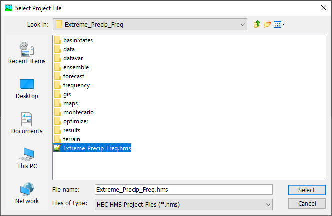
Launch HEC-HMS (version 4.12 beta 5 or later) and open the "Extreme Precip Freq" project by going to File > Open... and browsing to the location where you unzipped the initial project files. Select the "Extreme_Precip_Freq.hms" file.
In the Watershed Explorer in the upper left, expand the Basin Models node of the tree and click on the TuleRiver No Snow basin model to view the map of our watershed.
Note from the terrain model that the headwaters are in the high mountains, and everything concentrates down to the dam inflow site by dropping significantly in elevation.
While the TuleRiver No Snow basin model is selected, choose Parameters > Element Inventory from the main menu. Here you can see the cumulative drainage area for each element in the model. Our analysis will focus on the ReservoirInflow junction element, which is where flow is combined from the upstream elements and passed to our reservoir element. Note that the drainage area is about 390 mi2, so while this is not a large watershed, due to the terrain, there is likely to be high variability in the precipitation-frequency grids across the model domain. Close the Element Inventory.
Step 2: Import Precipitation-Frequency Data
We will use two different sources of precipitation-frequency data in this workshop. One is from NOAA Atlas 14 in .asc raster format, and the other is a set of data from a local study in .tif raster format.
Import 24-hour 1/1,000 AEP Grid from NOAA Atlas 14
NOAA Atlas 14 publishes point precipitation-frequency data for most of the country, with accumulation durations of 5 minutes up to 60 days, and with frequencies from 1/2 AEP to 1/1,000 AEP. We will get the rarest frequency from A14 to begin our extrapolation.
Download from PFDS
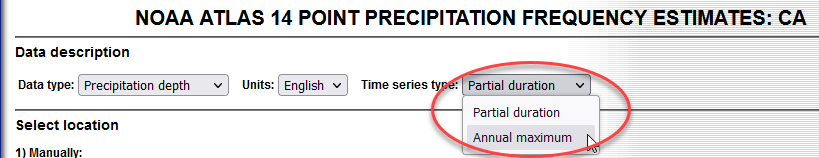
Go to the NOAA National Weather Service (NWS) Precipitation-Frequency Data Server website: https://hdsc.nws.noaa.gov/pfds/ and click on California on the map.

At the top of the new page that opens, there are three drop-down menus, and where it says "Time series type:" click the drop-down and choose "Annual maximum".
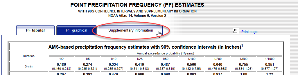
Scroll down on the page to the table with three tabs, and click on "Supplementary Information".
Under "II. PF in GIS Format" choose 1/1000 for annual exceedance probability and 24-hour for duration, and click "Submit".
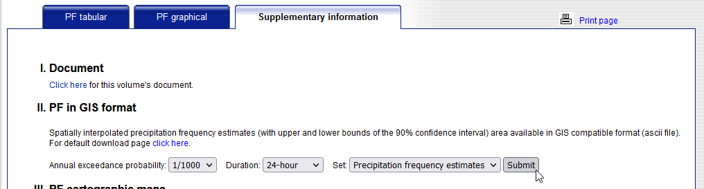
This will download a file called "sw1000yr24ha_ams.zip" which you should place in the data folder inside your HMS project. After downloading it, unzip the contents and ensure they are in that root data folder.
Import Grid to HEC-HMS Project
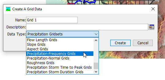
Create a new grid by going to Components > Create Component > Grid Data...
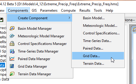
In the dialog that opens, first choose the Data Type to be Precipitation-Frequency Grids, then set the name to "A14 1000yr 24hr".
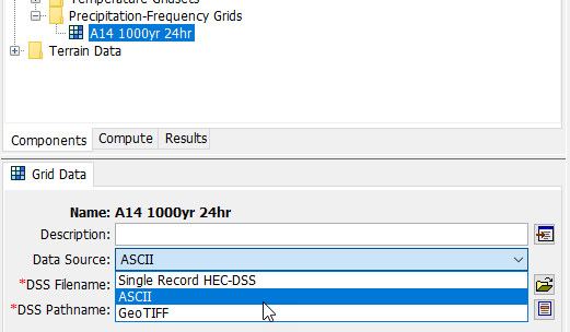
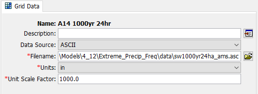
Next, go to the Watershed Explorer and expand Grid Data and Precipitation-Frequency Grids, and select the A14 1000yr 24hr grid. In the Component Editor, choose Data Source: ASCII, and a file chooser dialog will open. Navigate to your project data folder and choose the "sw1000yr24ha_ams.asc" file.
In the Component Editor, ensure the units are set to in and the unit scale factor to 1000.
Unit Scale Factors
Some raster data is stored in integer (whole number) format by taking the regular floating-point (decimal) values and multiplying them by a scale factor. For example, the floating-point value 0.501 might be stored as the integer 501 with a scale factor of 1,000. Typically, this value is reported in the dataset's metadata.
For Atlas 14, this scale factor is 1,000. If you use the NOAA Atlas 2 rasters from NOAA, the scale factor for those is 100,000.
If you use a floating-point (decimal) raster as the data source, you can leave the scale factor as 1.
Import 24-hour 1/5,000 and 1/10,000 AEP Grids from Site-Specific Precipitation-Frequency Study
To get beyond 1/1,000 AEP, usually some kind of dedicated regional frequency analysis with these frequencies in mind is required. We will use a hypothetical set of data representing potential 1/5,000 AEP and 1/10,000 AEP 24-hour storms for the watershed to extrapolate the rest of the way out.
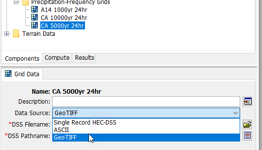
Two grids from a local precipitation-frequency study have been provided for demonstration in this workshop ONLY and should not be used for any other purpose. They are located in the project's data folder and are called "q5000_1d_clip.tif" and "q10000_1d_clip.tif". Use the same process to create two new grids of type Precipitation-Frequency Grids, calling one of them "CA 5000yr 24hr" and "CA 10000yr 24hr". In the component editor, choose "GeoTIFF" for the Data Source and choose the corresponding tif file in the data folder. Set the units to in and the unit scale factor to 1 for each of them.
Step 3: Import Temporal Patterns
Download 24-hour Temporal Patterns for the Region from PFDS
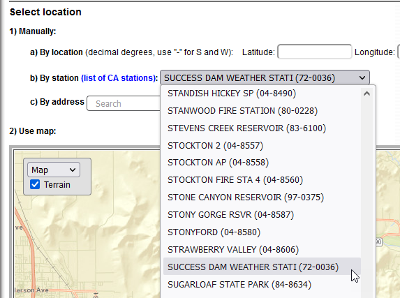
Returning to the PFDS webpage for CA (https://hdsc.nws.noaa.gov/pfds/pfds_map_cont.html?bkmrk=ca) near the top of the page, under "Select location" go to the drop-down menu and under "By station" choose SUCCESS DAM WEATHER STATI (72-0036).
Then, go back down to the "Supplementary Information" tab and under "IV. Temporal distributions" make sure 24-hour is selected and hit Submit.
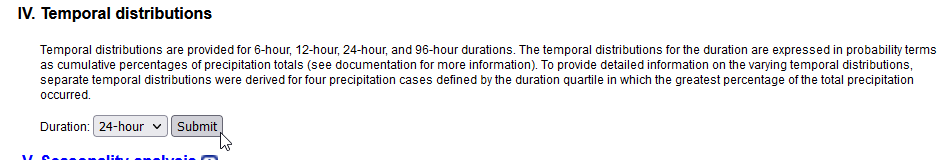
This will download a file called "ca_10_24h_temporal.csv" which you should place in your HEC-HMS project's data folder.
Import A14 Temporal Patterns
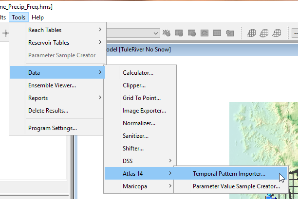
Under the Tools menu, choose Data > Atlas 14 > Temporal Pattern Importer...
In the dialog that launches, navigate to your project's data folder and select the "ca_10_24h_temporal.csv" you downloaded and press "Next".
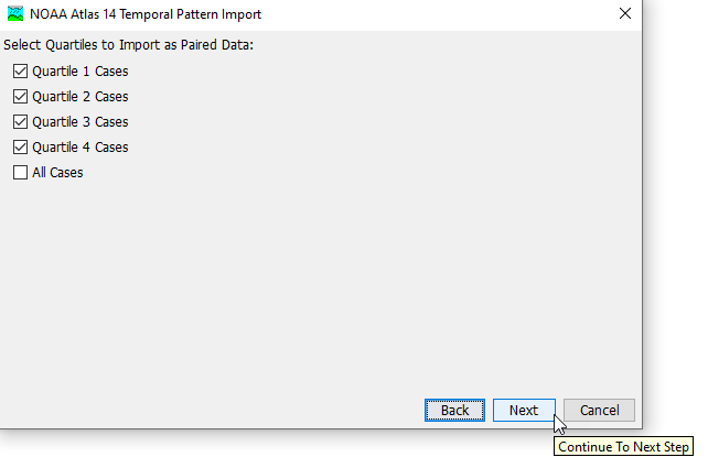
On the next window of the wizard, select the first four checkboxes (everything except "All Cases") and press Next.
On the next wizard step, it will automatically name the output DSS file and choose to put the file in your project's data folder. This is a good default so choose Next, then Close.
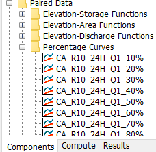
All of these curves will import as Percentage Curve Paired Data.
Step 4: Enter Area Reduction Information
A generalized depth-area-duration relationship (area reduction function) from HMR-59 (https://www.weather.gov/media/owp/hdsc_documents/PMP/HMR59.pdf) is provided for the Sierra region below. Create an area reduction function in HEC-HMS by choosing Components > Create Component > Paired Data...
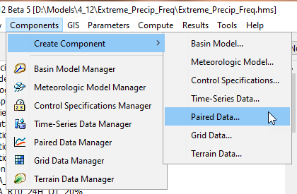
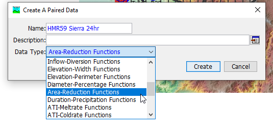
In the dialog that opens, first choose Data Type: Area-Reduction Functions, then name it "HMR59 Sierra 24hr".
After it is created, go to the Watershed Explorer and choose Paired Data/Area Reduction Functions and expand it to find the new curve. Click on it to open the Component Editor, and select the Table tab.
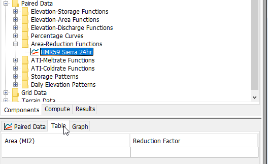
Paste in the below table reproduced from HMR-59 and save your project.
24-hour Generalized ARF for Sierra Region in HMR-59.
| Area (mi2) | 24 hr |
|---|---|
10 | 1 |
| 50 | 0.91 |
| 100 | 0.87 |
| 200 | 0.8275 |
| 500 | 0.77 |
| 1000 | 0.7225 |
| 2000 | 0.67 |
| 5000 | 0.59 |
| 10000 | 0.525 |
Step 5: Create Hypothetical Storm Met Models
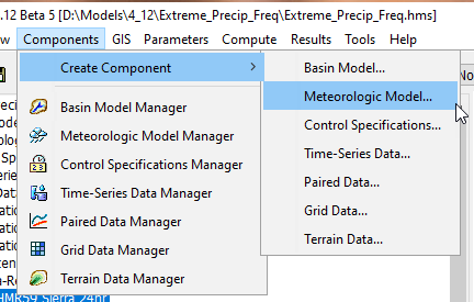
Create a new Meteorologic Model by going to Components > Create Component > Meteorologic Model...
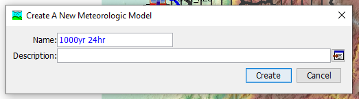
Call the new Meteorologic Model "1000yr 24hr" and select "Create".
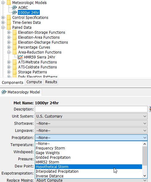
In the Watershed Explorer, under Meteorologic Models, select the new 1000yr 24hr Meteorologic Model. In the Component Editor, make sure the only method that is selected is "Hypothetical Storm" for the Precipitation method, all others should be turned off. Switching the Precipitation method will prompt you to make sure you want to change; select Yes.
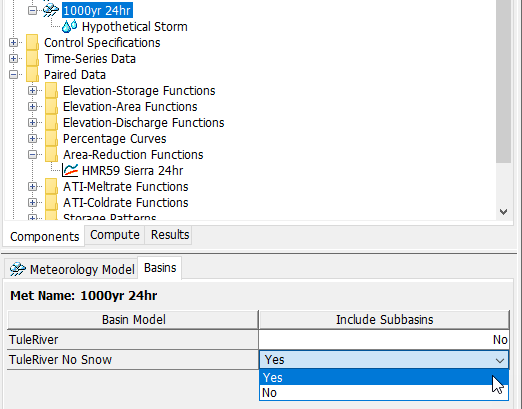
After switching the Precipitation method, a new tab will be added to the Meteorology Model Component Editor called "Basins". Click on this tab, then make sure the "Include Subbasins" option for the TuleRiver No Snow Basin Model is set to Yes.
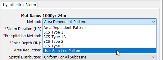
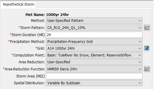
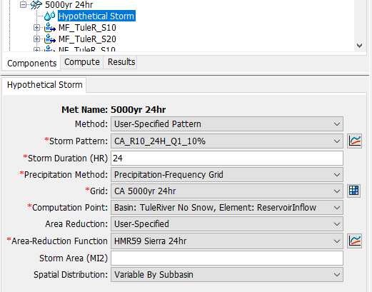
Expand the 1000yr 24hr Met Model and click on Hypothetical Storm. In the Component Editor, for Method, choose User-Specified Pattern.
The format of the Component Editor will change. Set up the Hypothetical Storm with the following options:
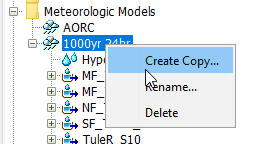
Create two more Meteorological Models by copying the 1000yr 24hr one using Right-Click, Create Copy... on the Met Model. Call the first one "5000yr 24hr" and the second one "10000yr 24hr".
Use the component editor to set the Grid to the correct grids (CA 5000yr 24hr and CA 10000yr 24hr, respectively).
Step 6: Create a Control Specification
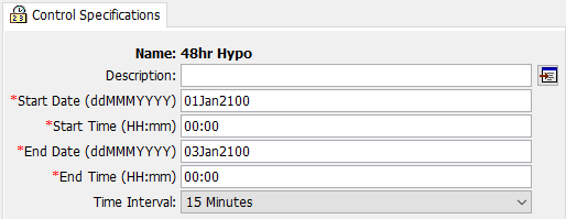
Create a new Control Specification by going to Components > Create Component > Control Specifications... and call it "48hr Hypo".
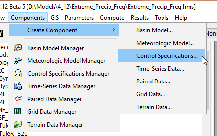
Open the Control Specification in the Watershed Explorer. Set the start date to "01JAN2100" and start time to "00:00", and the end date to "03JAN2100" and end time to "00:00". Leave the Time Interval set to 15 min.
Step 7: Run Frequency Events
Create Simulation Runs for Each Frequency
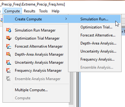
Create the first Simulation Run by going to Compute > Create Compute > Simulation Run... and call it "1000yr 24hr".
On the next three screens, choose the TuleRiver No Snow basin model, the 1000yr 24hr met model, and the 48hr Hypo control specification (pressing finish on the third screen).
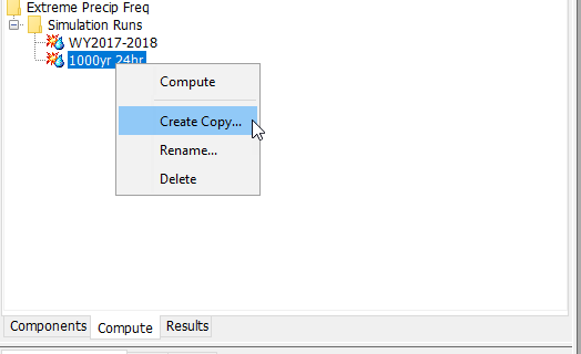
Create two copies of this Simulation Run called "5000yr 24hr" and "10000yr 24hr" by going to the Compute tab, selecting the 1000yr 24hr Simulation Run, right-clicking on it, and choosing "Create Copy..."
In the Compute tab, click on each of the two new Simulation Runs and edit the Met Model in the Component Editor so they link up with the 5000yr 24hr and 10000yr 24hr Met Models, respectively.
Run the Simulations
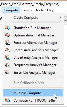
In the Compute menu, choose Compute > Multiple Compute...
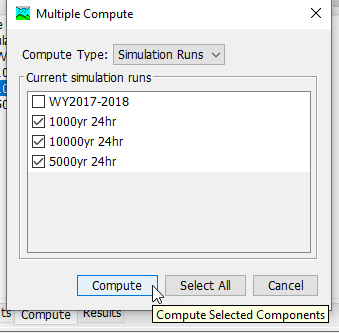
Check the three Hypothetical Storm Simulation Runs and press Compute.
Gather the Results
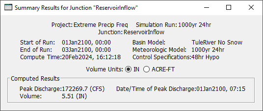
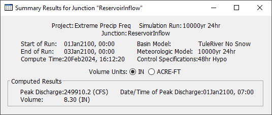
For each of the three frequency events you ran, record the peak discharges for the ReservoirInflow junction element (the computation point). Use the Summary Table to get the peak discharge for each of the frequency events.
Here are the summary tables for the 1/1,000, 1/5,000, and 1/10,000 events.

Step 8: Compare to Inflow Frequency Curve
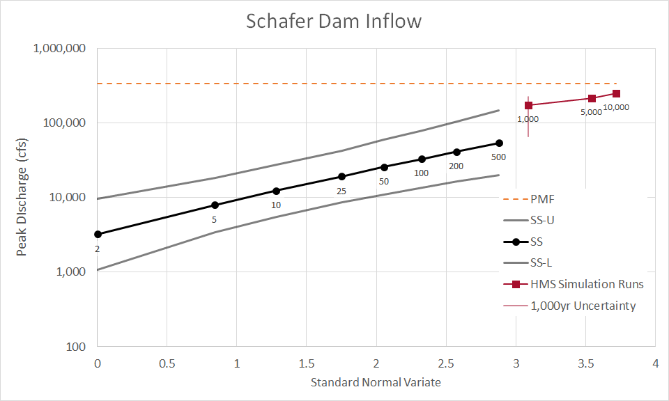
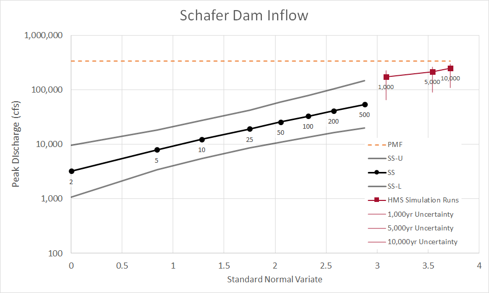
USGS StreamStats (https://streamstats.usgs.gov/ss/) was used to estimate a rough inflow-frequency curve and probable maximum flood (PMF) at the dam site. There is no USGS gage measure inflows to Schafer Dam, and in the absence of other data, such as computed inflows from the dam's operator, StreamStats produces a reasonable first guess at flow frequency for frequencies from 1/2 - 1/500 AEP.

The StreamStats report was used to create an Excel spreadsheet that can be used for comparing results from the HMS simulations. Download that spreadsheet here: schafer-dam_inflow-frequency_ws.xlsx

For the three frequency simulations you performed, put the discharge values in cells G11, G12, and G13 in the spreadsheet (the cells are highlighted in orange.) This will allow you to see where these three events plot relative to the frequency curve from StreamStats.
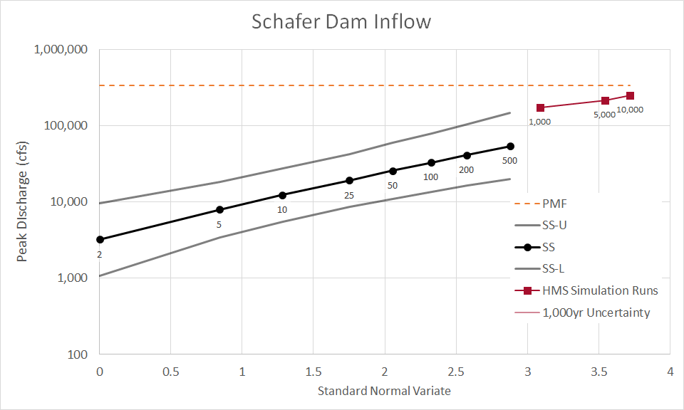
These events seem to run right along an imaginary line carried forward from the upper bound of StreamStats. It could be that our hypothetical storm assumptions, hydrologic model assumptions, or both, are biased on the high side when compared to StreamStats. StreamStats is not necessarily the truth, but the large discrepancy would be worth looking into.
Step 9: Run Uncertainty Analysis for Temporal Pattern and ARF for the 1/1,000 AEP Event
Temporal Pattern Uncertainty
Create Temporal Pattern Name Samples
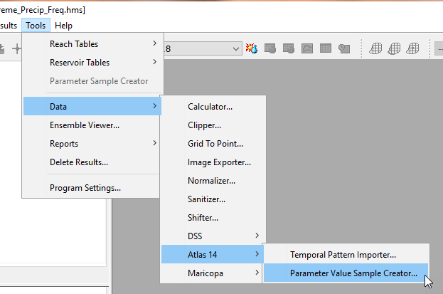
In the Tools menu, go to Data > Atlas 14 > Parameter Value Sample Creator...
In the new tool window that pops up, choose the "Storm Pattern" parameter.
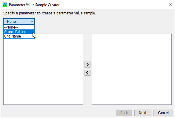
Select all the patterns on the left side by clicking on one of them and then using the keyboard shortcut CTRL+A. Then, select the ">" to move them all to the right side, and press "Next". On the next screen give the sample the name "A14 Temporals" and select "Next". On the next screen, select "Next", accepting the default choice to save the sample to the project DSS file. Press Next, then Close.
Sensitivity Due to Temporal Pattern
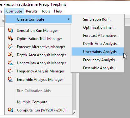
We will use the Uncertainty Analysis to see the effect of temporal patterns on the peak flow response of the 1/1,000 AEP event. Create a new Uncertainty Analysis by going to Compute > Create Compute > Uncertainty Analysis...
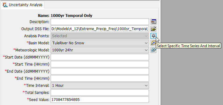
In the new window that opens, call the new analysis "1000yr Temporal Only" and select "Next >". On the next screen select TuleRiver No Snow for the basin model, and press "Next >". For the met model select 1000yr 24hr and press "Finish".
On the Compute tab, expand the folder for Uncertainty Analyses and choose the new 1000yr Temporal Only analysis. Next to the Analysis Points click on the gear icon to open the output selection options.
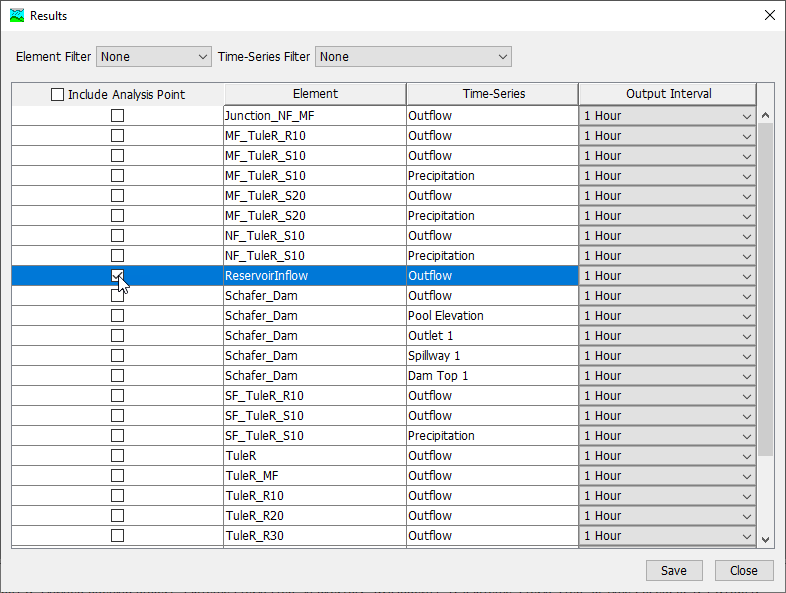
In that window choose the Outflow timeseries for the ReservoirInflow element, and press "Save" and then "Close".
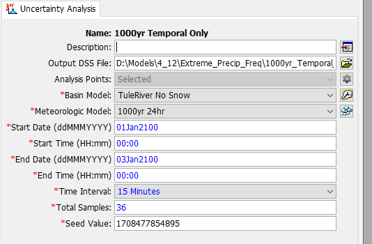
Enter a start date of "01Jan2100" and start time of "00:00", then an end date of "03Jan2100" and end time of "00:00". Set the time interval to 15 minutes. Select 36 total samples (there are 36 total curves in the A14 set). Let the Seed Value stay whatever value HMS generates (it will be different than the one you see below). Save your project.
Back on the Compute tab, right click on the 1000yr Temporal Only Uncertainty Analysis and select "Add Parameter". A new node will be added to the tree called "Parameter 1". Click on that new node.
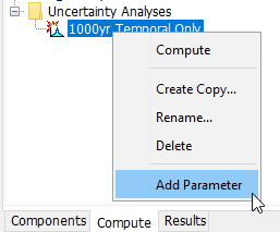
For Element choose "--Precipitation Parameters--". For Parameter choose "Hypothetical Storm - Storm Pattern". Then, save the project. Leave the Method option as "Specified Values - Sequential Loop" and choose A14 Temporals for Parameter Value. Then, save the project.
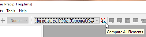
In the toolbar, select the Uncertainty: 1000yr Temporals Only simulation and click the button to the right to Compute All Elements. The model will run 36 times (specified by the Total Samples in the Uncertainty Analysis controls) and will take under a minute to complete.
On the Results tab, expand Uncertainty Analyses, expand the 1000yr Temporal Only simulation, then click on ReservoirInflow. It will expand to show four elements, click on the Outflow graph first. The result will be a summary hydrograph that shows for each timestep in the simulation window what the min, mean, and max flow are, and a +/- 1 standard deviation range around the mean. Next, click on the Maximum Outflow table to see the peak discharge from each of the 36 simulations and note the range of results due to the time pattern uncertainty.
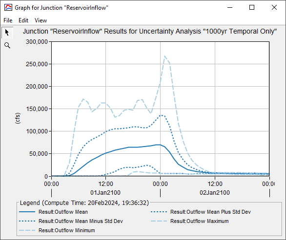
The peak discharges average about 141,300 cfs, with a range from about 57,500 cfs to 272,000 cfs!
Area Reduction Uncertainty
Previously, we used the generalized HMR59 area reduction curve for the Sierra region. The dam could reasonably also be considered to be in the Central Valley region. Additionally, one storm used in HMR59 fell somewhere near the dam: Storm 1007.


We will consider the uncertainty in the 1/1,000 AEP 24 hour storm by adding in ARF uncertainty considering these two other curves.
Follow the previous procedures to create two new Area Reduction Functions called "HMR59 CV 24hr" and "Storm 1007 24hr".
24-hour Generalized ARF for Central Valley Region in HMR-59.
| Area (mi2) | 24 hr |
|---|---|
10 | 1 |
| 50 | 0.915 |
| 100 | 0.865 |
| 200 | 0.81 |
| 500 | 0.72 |
| 1000 | 0.645 |
| 2000 | 0.555 |
| 5000 | 0.42 |
| 10000 | 0.3 |
24-hour Computed ARF for Storm 1007 in HMR-59.
| Area (mi2) | 24 hr |
|---|---|
10 | 1.000 |
| 50 | 0.917 |
| 100 | 0.864 |
| 200 | 0.839 |
| 500 | 0.747 |
| 1000 | 0.640 |
| 2000 | 0.508 |
| 5000 | 0.345 |
| 10000 | 0.256 |
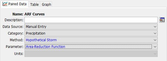
Next, create a new Paired Data of type "Parameter Value Samples" and call it "ARF Curves".
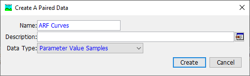
In the Watershed Explorer, under Paired Data/Parameter Value Samples, click on the new Paired Data to open the Component Editor. In the editor, change the Method to "Hypothetical Storm" and the Parameter to "Area-Reduction Function". Save the project.
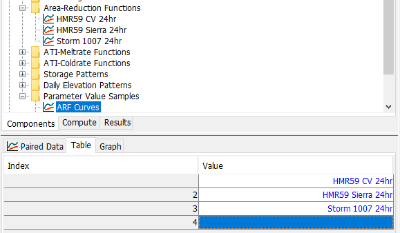
Change to the Table tab. In the Value column, add the names of your three ARF Paired Data: HMR59 CV 24hr, HMR59 Sierra 24hr, and Storm 1007 24hr.
Note
In a real study you would consider many ARFs in your uncertainty analysis, probably from a sample of DAD tables computed for storms that make sense for the watershed you are testing.
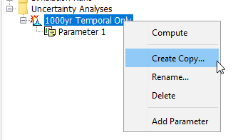
Go to the Compute tab in the Watershed Explorer, and right-click on your existing 1000yr Temporal Only Uncertainty Analysis, and select "Create Copy..." and in the Copy dialog call the new analysis "1000yr ARF Only".
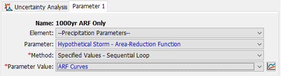
Click on the new 1000yr ARF Only Uncertainty Analysis so that it expands the parameter list. Click on Parameter 1 and change the Parameter to "Hypothetical Storm - Area-Reduction Function". Then, change the Parameter Value to "ARF Curves".
Since there are only 3 curves in our ARF curve sample, we would really only need 3 runs to see the spread in the results. The HEC-HMS Uncertainty Analysis has a minimum of 10 samples. Click on the 1000yr ARF Only Uncertainty Analysis and in the Component Editor, change the Total Samples parameter to 12 (the smallest multiple of 3 greater than 10).
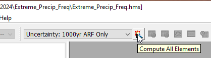
Run the Uncertainty Analysis by going to the top toolbar, selecting Uncertainty: 1000yr ARF Only and then the "exploding hydrograph" icon.
After it completes (15-30 seconds at the most), switch to the Results tab in the Watershed Explorer, expand the Uncertainty Analysis folder and select the 1000yr ARF Only Uncertainty Analysis. Then, select the ReservoirInflow junction element and take a look at the Outflow graph and the Maximum Outflow table. You can also check the "Parameter 1" table under the Uncertainty Analysis to see which curves correspond to which results.
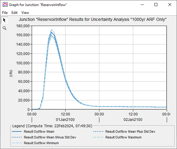
Just looking at the uncertainty from these three ARFs alone, the peak discharge varies between about 157,700 cfs and 172,300 cfs with the single temporal pattern we assumed in the original Meteorologic Model. From the parameter samples, it appears that the Sierra generalized ARF curve produces the highest result, and the CV generalized curve produces the lowest.
Combined Temporal Pattern and ARF Uncertainty
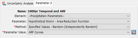
Finally, we will combine the effects of temporal pattern and area reduction uncertainty in a third uncertainty analysis. Start by creating a copy of the 1000yr Temporal Only Uncertainty Analysis and call it "1000yr Temporal and ARF". Right-click on the newly created Uncertainty Analysis to add a second parameter. Click on Parameter 2 and set its Element to "--Precipitation Parameters–", the Parameter to "Hypothetical Storm - Area-Reduction Function", and the Method to "Specified Values - Random (Independently Random)". Save the project, then select "ARF Curves" for the Parameter Value.
Click on Parameter 1 and change the Method to "Specified Values - Random (Independently Random)". This will clear the Parameter Value selection, and you should re-select A14 Temporals. Then, save the project.
Between the 36 temporal patterns and 3 ARFs there are 108 combinations of the two. We want enough samples to cover all these possibilities, so set the Total Samples for the Uncertainty Analysis to 200 by clicking back on the Uncertainty Analysis tab in the component editor. Then, run the simulation. It should take about 3-5 minutes at the most.
After the simulation completes, check the results on the Results tab in the Watershed Explorer. Look at the Maximum Outflow table to get a sense of how much the results from running the 1/1,000 AEP 24-hour storm can vary.
In the results spreadsheet we used before, copy the 200 values out of the Maximum Outflow table and paste them into the spreadsheet on worksheet 1000yr beginning in cell B2 (the cell highlighted in red.) The summary statistics will automatically compute for this set of data, and the frequency curve plot will update with a line representing the 5%-95% range of the results.
The mean result from these 200 iterations is about 136,500 cfs (median 133,500 cfs). The range is between 51,800 cfs and 267,600 cfs!
Final Question: when running precipitation-frequency events to generate a flow frequency curve, what is the impact of making an assumption about the temporal pattern or area reduction function for the event? What other sources of uncertainty did we ignore in the above exercises?
Usually we assume a single temporal pattern and single area reduction function when running a frequency event. This can vastly overstate our confidence in the answer; in other words, we understate the uncertainty. Real storm events can exhibit incredible variability in spatial and temporal behaviors, which we mostly represent with a single representative ARF and temporal pattern.
In this exercise we assumed that the uncertainty in the 1/1,000 AEP 24-hour depth was zero. If you check the tables in Atlas 14, you can see that there are estimates for uncertainty in the frequency depths reported as a 90% confidence interval. The size of this range means that the maximum flow results are probably very sensitive to this parameter.
We assumed the storm was 24 hours in duration. The frequency rainfall we apply and the ARF we select is dependent on the duration we have chosen. In reality, storms have varying durations. We typically select a duration that is longer than the watershed's time of concentration and has precipitation-frequency and ARF information, with 24 hours being one of the most common.
We assumed a single storm spatial pattern that follows the spatial pattern of the 1/1,000 AEP 24-hour rainfall when it was distributed to the subbasins in the model. A real storm that produces a 390 mi2 1/1,000 AEP 24-hour rainfall may manifest in any number of spatial patterns. The distribution of this rainfall in space may be highly variable, and due to the runoff response of the watershed, may lead to different results in the peak discharge.
We assumed that the same temporal pattern occurred at all the subbasins in the model at the same time. This may not be realistic given how storms track across the watershed, and may impact the response at the inflow of the dam. However, this is hard to assess without using totally different hypothetical storm methods like Stochastic Storm Transposition.
We assumed that the same ARF was applicable to all three of our frequency events, when in reality ARF may be a function of AEP in addition to duration. We would need to sample separate sets of ARF for each frequency in order to capture this effect, which is challenging due to a lack of data.
Finally, we assumed that the 390 mi2 1/1,000 AEP 24-hour rainfall could be computed as the average of the point precipitation-frequency product everywhere in the watershed and then reduced using an ARF. This is also a challenging assumption to address by modeling in an uncertainty analysis.
Can you think of any other assumptions?
Step 10 (Optional): Run Uncertainty for 1/5,000 and 1/10,000 AEP Events
Repeat the above procedure by duplicating the 1000yr Temporal and ARF Uncertainty Analysis and changing the Meteorologic Models so that they correspond to the 1/5,000 and 1/10,000 AEP events. No other settings need to be changed.
In the plotting spreadsheet, you can paste the results on worksheets 5000yr and 10000yr in cell B2 and the plot will automatically update with the new data.
Considering just the temporal and ARF uncertainty, it seems like the choices we made in the original model were probably on the conservative end, and that the 5%-95% uncertainty range computed using the uncertainty analysis places our original scenario towards the top of that range.
Download the final files here: Extreme_Precip_Freq_Final.zip