Download PDF
Download page Applying the HMR52 Storm Meteorologic Model in HEC-HMS.
Applying the HMR52 Storm Meteorologic Model in HEC-HMS
Overview
This tutorial will guide you through the process of applying the HMR52 meteorologic model in HEC-HMS to manually maximize the Probable Maximum Precipitation (PMP) precipitation upstream of Sayers Dam. You will be creating a new HEC-HMS project by georeferencing an existing watershed polygon. The goal of this task is to create a PMF basin model, set up the HMR52 Storm meteorologic model, run a simulation with the PMP event, and then use the Optimization Trial to maximize precipitation over a watershed. The following steps show you how to create a basin model, set the coordinate system to Albers Equal Area, import GIS features (subbasins), and define the loss, transform, and baseflow parameters. The steps also show the process of setting up a HMR52 Storm meteorologic model, defining control specifications, and creating, running, and reviewing the simulation.
Data
Download the watershed polygon and stream line shapefile here: PMP_Workshop_Initial_2024.zip
Steps
Launch HEC-HMS. From the File menu select New... to create a new project. Call the project PMP Workshop and make sure the default unit system is U.S. Customary.
Start with the creation of a new basin model for the PMP analysis. Go to the Components menu and select Create Component | Basin Model... Name the model PMF_Sayers and click Create.
Before importing the shape file, the coordinate system for the basin model must be defined. To set the coordinate system, first activate the PMF_Sayers basin model in the Watershed Explorer by selecting Basin Models | PMF_Sayers. From the GIS menu select Coordinate System. In the Coordinate System panel click Browse. Navigate to where you extracted the zip file with the watershed polygon and stream line shapefil. Select the Basin_Albers.shp file and click Select. The coordinate system for PMF_Sayers should now be populated with Well Known Text (WKT) exhibiting an Albers Equal Area Projection as shown below. Click Set to establish the coordinate system for PMF_Sayers.
Question 1: Why would an Albers Equal Area projection be appropriate for a PMP analysis? Can you think of other projections that would be appropriate?
The Albers Equal Area projection is an equal-area projection and preserves area. Equal-area projections will result in a better approximation of total water volume than projections such as conformal, compromise, equidistant, etc. The second question is a trick question. All future analysis should use the standard MMC projection.
With the coordinate system set, the subbasin upstream of Sayers Dam can be imported as a GIS feature. From the GIS menu select Import Georeferenced Elements. Make sure Element Type is set to Subbasins and click Next. Browse for Basin_Albers.shp, select the file for import, and click Next. Select the field definition NAME to identify the attribute containing the name for the subbasin, and then click Finish. Now view the newly imported GIS element Bald Eagle HW as shown below.
The map panel has sparse detail and would benefit from additional map layers for visualization purposes. Make sure in the Watershed Explorer panel that the PMF_Sayers basin is still selected. From the View menu select Map Layers… | Add.... Select Reach_Albers.shp and click Select. The current map layers should now include Reach_Albers, as shown below, and the Map Layers editor can be closed.
Now that the basin model includes elements and map layers, it is time to populate the parameters for the Bald Eagle HW subbasin element. In the Watershed Explorer select the PMF_Sayers basin node. In the Component Editor, set the Unit System for the basin model to U.S. Customary. Expand the PMF_Sayers basin model and select the Bald Eagle HW subbasin. The Component Editor will activate as seen in the first figure below. On the Subbasin tab, set the loss, transform, and baseblow methods to Initial and Constant, Clark Unit Hydrograph, and Recession respectively. Now the loss, transform and, base flow parameters will need to be specified as shown in the next three figures below. Select the Loss tab and specify the loss parameters, Initial Loss (IN) = 0.2 and Constant Rate (IN/HR) = 0.1. Select the Transform tab and specify the transform parameters, Time of Concentration (HR) = 9 and Storage Coefficient (HR) = 9. Select the Baseflow tab and specify baseflow parameters, Initial Discharge (CFS) = 1, Recession Constant = 0.7, and Ratio = 0.05. With the parameters set, it is now time to configure an HMR52 Storm meteorologic model.


HMR 51 and 52 Background Information
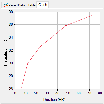
Hydrometeorological Report 51 (HMR51) contains the PMP index maps for the Eastern U.S. and Hydrometeorological Report 52 (HMR52) contains information about the application of the PMP depths to a watershed. Figures 18 – 47 in HMR51 contain depth-area-duration (DAD) PMP index values for the area east of the 105th meridian in the United States. The PMP documents have been digitized by the national weather service (NWS) (https://www.weather.gov/owp/hdsc_pmp). The below table contains most of the DAD PMP values for the Sayers Dam watershed. It is good practice to plot the DAD values in a plot similar to the one below to catch any mistakes when extracting the information for your watershed.
Question 2: What is the PMP depth for the 6-hour 5,000 square mile storm area using the HMR51 document?
Using HMR51 Figure 33, interpolate between the isohyets given that Sayers Dam is located at approximately 41 N and 77.5 W. The 6-hour 5,000sqmi PMP depth for the Sayers Dam watershed is approximately 7.80 inches.
Depth-area-duration PMP values for the Sayers Dam watershed
| Area (sqmi) | 6-hours | 12-hours | 24-hours | 48-hours | 72-hours |
|---|---|---|---|---|---|
| 10 | 26.14 | 29.95 | 32.55 | 35.82 | 37.38 |
| 200 | 17.81 | 21.16 | 23.94 | 27.01 | 28.05 |
| 1000 | 12.86 | 15.97 | 18.72 | 21.30 | 22.57 |
| 5000 | 10.92 | 13.22 | 15.94 | 17.21 | |
| 10000 | 6.04 | 9.13 | 10.97 | 13.58 | 14.99 |
| 20000 | 4.23 | 7.18 | 9.02 | 11.73 | 12.74 |

With the above DAD PMP values derived from HMR51, a meteorologic model for a PMP analysis can be created and populated in HEC-HMS. Navigate to Components | Create Component | Meteorologic Model. Name the model PMP and click Create. The meteorologic model has been added to the project and can be found in the Watershed Explorer as shown below.
In the Watershed Explorer select PMP to activate the Component Editor. Under the Meteorology Model tab, change the Precipitation method to be HMR52 Storm. When prompted to change methods click Yes. Set the Unit System to U.S. Customary. The Meteorology Model should now be configured for HMR52 storm inputs as shown below.
The duration-precipitation functions must be added to completely populate the required HMR52 Storm information. These functions are defined as paired data. Go to the Components menu and select Paired Data Manager. Under Data Type select Duration-Precipitation Functions from the dropdown menu. Click New... and name the first paired data set 10 sq mi, and click Create as shown below. Repeat this process for the remaining storm areas: 200 sq mi, 1000 sq mi, 5000 sq mi, 10000 sq mi, and 20000 sq mi. 
Once the duration-precipitation functions are created, they can be populated with the data found in the above table (see step 6). In the Watershed Explorer navigate to Paired Data | Duration-Precipitation Functions and select 10 sq mi paired data entry to activate the Component Editor. On the Paired Data tab, set the units to HR : IN. Select the Table tab and populate the table with the appropriate values as seen in the figure below. Repeat the process for the remaining paired data entries: 200 sq mi, 1000 sq mi, 5000 sq mi, 10000 sq mi, and 20000 sq mi. Note: it may help to copy and paste the left column containing the duration (hr) values into subsequent functions.
Now that the duration-precipitation functions are populated, the HMR52 Storm meteorologic model can be parameterized. In the Watershed Explorer select Meteorologic Models | PMP | HMR52 Storm to activate the Component Editor. On the HMR52 Storm tab, assign the X and Y coordinates for the storm center. The X and Y coordinates can be estimated using GIS. Use coordinates 4942618 and 6985660 as starting values.
Continue filling in the HMR52 Storm tab with the following information found in the HMR 52 document: Preferred Orientation (DEG) = 211, Orientation= 211, Peak Intensity: Hours 36 to 42, and 1 to 6 Ratio = 0.305, and Area (MI2) = 350. Link the Area to the appropriate Duration-Precipitation Functions as shown below.
With the basin model and meteorological model complete, the control specification can be created for the PMF simulation. Go to the Components menu and select Create Component | Control Specifications. Name the new control specification PMF Event and click Create.
With the control specification created, go to the Watershed Explorer and select the Control Specifications | PMF Event node to activate the Component Editor. The Start Date, Start Time, End Date, End Time, and Time Interval will need to be specified as shown below. Set the control specifications time window to be 01Jan1999 00:00 to 08Jan1999 00:00 and a time interval of 15 minutes.
Lastly, create the simulation run. From the Compute menu select Create Compute | Simulation Run. Name the new simulation run PMF Sayers and click Next. Select PMF_Sayers as the basin model and click Next. Select PMP as the meteorologic model and click Next. Select the control specification PMF Event and click Finish.
The simulation run is created and can be computed. From the Compute Toolbar select Run: PMF Sayers as shown below. Click the "exploding rain drop" compute button to run the simulation.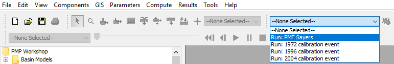
Review results of peak flow, flow volume, and precipitation volume and record the results. In the Watershed Explorer, click on the Results tab and expand the PMF Sayers node and then the Bald Eagle HW element node as seen in the figure below. Be sure to check out the Graph and Summary Table results and note the maximum peak flow computed for the Bald Eagle HW subbasin element. 
Now navigate to the Watershed Explorer pane under Meteorologic Models and select PMP | HMR52 Storm and experiment with different storm properties to maximize peak discharge at the Bald Eagle HW subbasin outlet. Try five additional scenarios (parameter combinations) and track your results. Focus on slight adjustments to the X and Y Coordinates, Orientation, and Area.
Map Pane Coordinates
Hovering the mouse cursor over the Basin Map Pane will show the X and Y coordinates at the cursor's current location.

| Scenario | X | Y | Orientation | Area (MI2) | Peak Flow (CFS) |
|---|---|---|---|---|---|
| 1 | 4942618 | 6985660 | 211 | 350 | 245,276 |
| 2 | |||||
| 3 | |||||
| 4 | |||||
| 5 | |||||
| 6 |
Question 3: What combination of Area and Orientation parameters produced the largest peak flow?
As the storm parameters are adjusted, an orientation of 226 deg and an area around 300 sqmi should produce the largest peak inflow, similar to the below summary results.

Create a new Optimization Trial by going to Compute > Create Compute... > Optimization Trial. Call the new trial "Maximum Precipitation". Use the PMF_Sayers basin model and PMP meteorologic model and click Finish on the last screen to create the trial.
On the Compute tab of the Watershed Explorer, expand the Optimization Trials node, and select the Maximum Precipitation trial. Set the start date and time to 01Jan1999 00:00 and the end date and time to 08Jan1999 00:00. Set the time interval to 15 Minutes.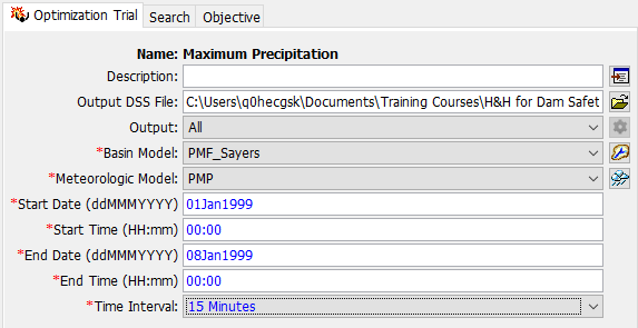
In the Component Editor change to the Objective tab. For Goal select Maximization. Set the Time-Series option to Precipitation and save the project.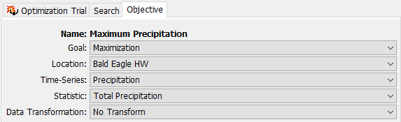
Switch to the Search tab and change the Method to Differential Evolution. Set the Min Iterations to 40.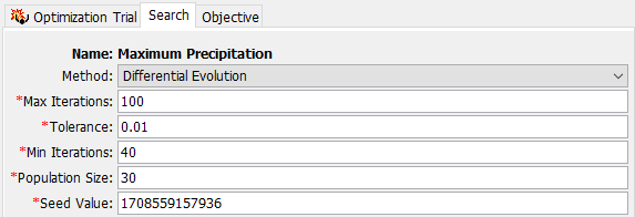
In the Watershed Explorer right-click on the Maximum Precipitation trial and select "Add Parameter". Repeat this 3 more times for a total of 4 parameters.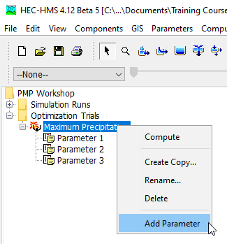
For the four parameters:
- Element: --Precipitation Parameters--; Parameter: HMR52 Storm - X Coordinate; accept default initial/min/max values
- Element: --Precipitation Parameters--; Parameter: HMR52 Storm - Y Coordinate; accept default initial/min/max values
- Element: --Precipitation Parameters--; Parameter: HMR52 Storm - Area; accept default initial value, set min to 10 sq mi and max to 2000 sq mi
- Element: --Precipitation Parameters--; Parameter: HMR52 Storm - Orientation; accept default initial/min/max values
Optimization Parameter Ranges
When using an optimization trial operationally (and not just for a workshop) it is important to set thoughtful, meaningful ranges for your parameters to make sure the search is bounded and goes quickly. In this situation, we are lucky that the default ranges are good enough to start a trial.
In the upper ribbon, select Trial: Maximum Precipitation and click on the "exploding local minimum" icon to its right to run the trial.
Each evaluation should be very fast. Due to our settings, the model will run at minimum 1200 evaluations (40 minimum iterations * 30 population size). This should complete in 1-2 minutes at the most.
In the Watershed Explorer, go to the Results tab and choose the Maximum Precipitation trial.
Question 4: Look at the Objective Function graph which tells you how the search for maximum precipitation progressed. Does it seem to converge on a value?
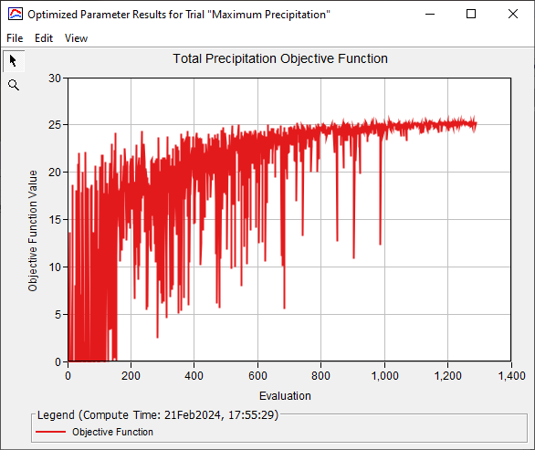
The trial seems to converge on a value a little higher than 25 inches.
Question 5: Look at the parameter trace values for each of the four parameters. Do they each seem to converge on a value?
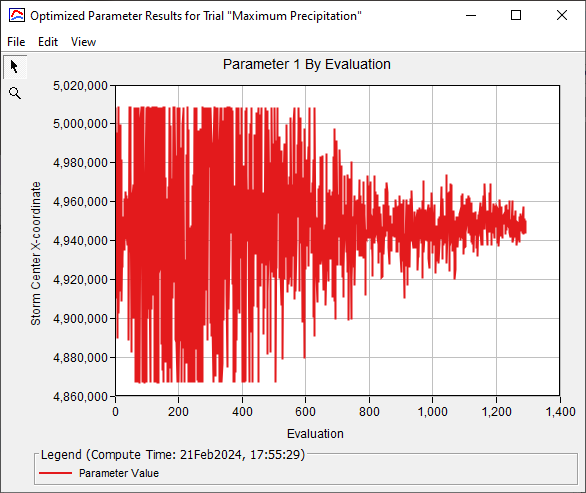
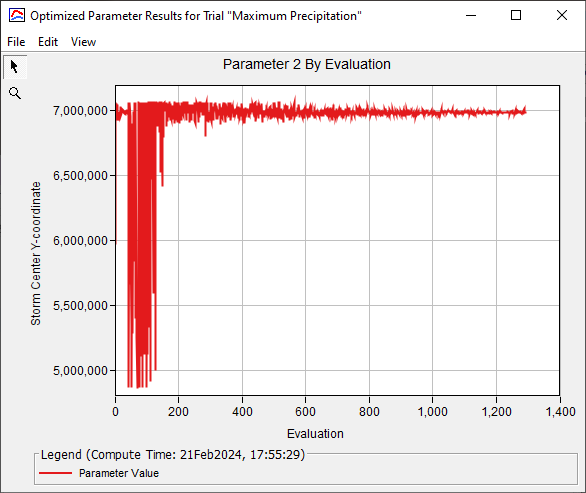
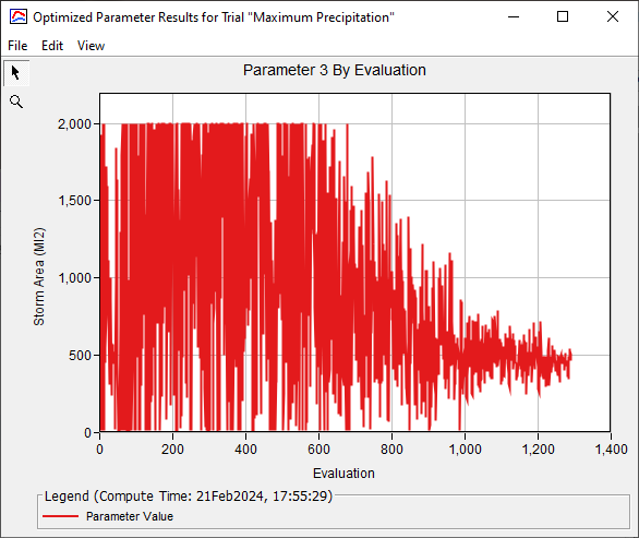
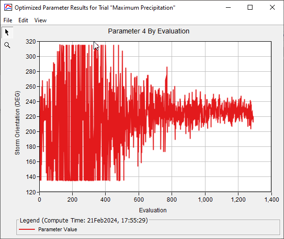
Each parameter starts out fairly noisy, but the range of the search gets narrower and narrower as the search progresses. Each seems to be converging towards a final answer. You will notice that the initial range for Parameter 2 (Y value) is much too large and better constraining would speed up the search a lot.
The smaller and smaller variance in the objective function indicates that the last bit of noise in each of these parameters may not be very sensitive in affecting the actual maximization.
Finally, look at the Optimized Parameters table. Note the values for the four parameters that maximize total precipitation over the watershed. Click on the Bald Eagle HW subbasin element under the trial, and click on the Summary Table.
Question 6: Did maximizing total precipitation also maximize peak discharge? Is the peak discharge value higher than before?
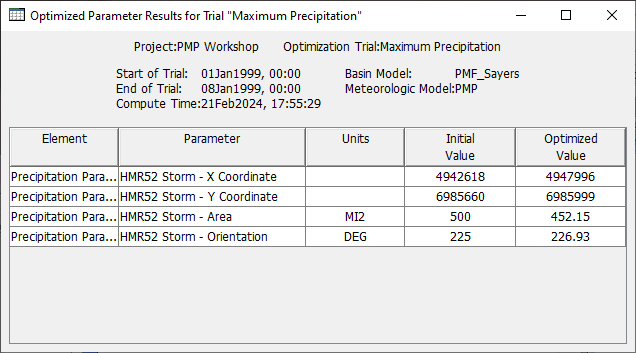
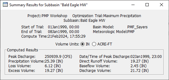
This process pushed the peak discharge over 250,000 cfs. Here you can see the maximized precipitation volume is 25.39 inches.
Link to a completed version of the workshop: PMP_Workshop_Final_2024.zip