Download PDF
Download page Using the Optimization Trial with an HMR52 Storm Meteorologic Model.
Using the Optimization Trial with an HMR52 Storm Meteorologic Model
Overview
HEC-HMS includes an optimization trial that can be configured to determine the maximum inflow into Sayers Dam through optimization of the HMR52 Storm meteorologic model parameter set. The optimization trial replaces the need for many manual iterations of running simulations to determine the optimal HMR52 Storm parameter set. The parameters that will be adjusted in the optimization trial are Orientation, Area, and the X and Y coordinates. In the prior section, the focus was around the Bald Eagle HW subbasin element. In this section, the focus will be around the entire collection of subbasins that are upstream of Sayers Dam. Subbasins downstream are also included in order to compute the residual runoff from a PMP occurring upstream of the dam.
Data
If you are just finishing the previous section on Applying the HMR52 Storm Meteorologic Model in HEC-HMS 2022, you may continue to use that model. Otherwise, download the initial model files here - PMP_Optimization_Workshop_Initial.zip
Steps
- If you are continuing from the previous section, you may skip to step 2. Otherwise, launch HEC-HMS. From the File menu select Open... | Browse to navigate to the downloaded project on your local computer and click the PMP_Workshop.hms file. Click Select to open the project.
- First start by creating a simulation for the Bald Eagle Creek basin model. From the Compute menu, select Create Compute | Simulation Run. Name the run PMF_BEC and click Next. Select the basin model PMF_BEC and click Next. Select the meteorologic model PMP and click Next. Select the control specification PMF Event and click Finish.
Select the PMF_BEC basin model in the Watershed Explorer and then at the Compute Toolbar select Run:PMF_BEC. Click the "exploding rain drop" button to compute. The PMF_BEC simulation run that was just computed incorporates additional subbasins, reservoirs, and routing reaches and can give insight into flows downstream of Sayers Dam. View results at the Sayers Dam reservoir element.

Question 1: What is the peak stream flow directly downstream of Sayers Dam? How does this compare to the inflow into Sayers Dam?
From the below results figure, we see a reduction in the hydrograph peak for the outflow of Sayers Dam. The peak outflow is around 180,000 cfs and the peak inflow is around 210,000 cfs. The dam reduces the peak flood event.

- Now that the simulation for PMF_BEC basin is confirmed operational, an optimization trial can be developed. The optimization trial will help us quickly determine the storm location, orientation, and area that leads to a maximum flow into the Sayers Dam reservoir element. From the Compute menu select Create Compute | Optimization Trial. Name the optimization trial Optimization PMP and click Next. Select the basin model PMF_BEC and click Next. Select the meteorologic model PMP and click Finish.
- The optimization trial has been created and the time window can be configured. Navigate to the Watershed Explorer and click the Compute tab. Expand the Optimization Trials node and select Optimization PMP. The Component Editor will activate and the Optimization PMP trial can be parameterized. Set the time window to be 01Jan1999 00:00 to 08Jan1999 00:00 and a time interval of 15 minutes as shown below, which is the same time window used in the previous section.

- Switch to the Search tab to assign the Method: Simplex, Max Iterations: 150, and Tolerance: 0.1 as shown below. In this case, the tolerance is representative of the change in the discharge value (CFS) between iterations.

- Set the objective of the optimization trial by switching to the Objective tab. Set Goal: Maximization, Location: Pool HW, Time-Series: Discharge, and Statistic: Peak Discharge as shown below. The Optimization is now configured to maximize the peak discharge into Sayers Dam.

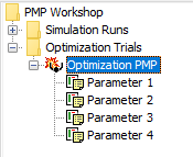
- In the Watershed Explorer, right click on the Optimization PMP node and select Add Parameter. A new parameter will be added to Optimization PMP. Continue adding three more parameters for a total of four as shown below.
With the four parameters elements created, the X and Y coordinates, Orientation, and Area can be specified for each parameter. In the Watershed Explorer select Optimization PMP | Parameter 1 to activate the Component Editor. Then select Element: --Precipitation Parameters--, Parameter: HMR 52 Storm – X Coordinate. The Initial Value should reflect what was specified in the PMP meteorologic model and Minimum and Maximum values should be already populated accordingly, as shown below. Repeat this process for Parameters 2-4, selecting the Y coordinate, Orientation, and Area parameters. For the Area parameter specifically, override the default Minimum and Maximum values and specify a Minimum of 100 miles and a Maximum of 1000 miles.

Note
The initial value for each parameter defaults to settings within the HMR52 Storm meteorological model. In this example, the initial value for the X coordinate, Y coordinate, Orientation, and Area are each populated based on the PMP meteorological model.

- The optimization trial is now parameterized and can be computed. Go to the Compute Toolbar and select Trial: Optimization PMP and click the Trial Compute button.
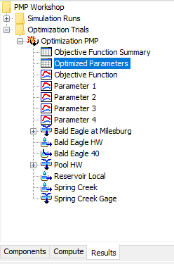
Reviewing optimization results is easily accomplished by going to the Watershed Explorer and selecting the Results tab. Navigate to the Optimization Trials directory and select Optimization PMP. Review the Objective Function Summary and Optimized Parameters table and other graphs as shown in the below figure.
Question 2: How do the optimized parameters compare to the parameters selected manually in the previous section? Are you surprised by the result?The optimized results are shown in the figure below. Ideally, the optimized values shown should be similar to what were observed previously.


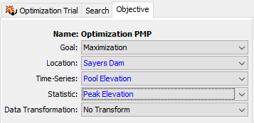
Question 3: Will changing the Objective tab parameters, Time-Series: Pool Elevation and Statistic: Peak Elevation as shown below, dramatically affect the optimized parameters? If Sayers Dam Peak Elevation is selected, then the tolerance should be lowered from 0.1 to 0.0005. Try different starting values for the storm parameters to see if an improved “optimal” HMR52 storm parameter set can be found by the optimization trial.
Note
When running an optimization trial in HEC-HMS, if the algorithm converges too quickly (in just a few iterations) try lowering the tolerance and re-computing.
The optimization will change slightly with the peak elevation objective. The results are shown in the below figures.


Download the final model files here - PMP_Optimization_Workshop_Final.zip