Download PDF
Download page Applying the New Linear Reservoir Baseflow Option with 2D Surface Flow.
Applying the New Linear Reservoir Baseflow Option with 2D Surface Flow
The purpose of this tutorial is to provide information about the new "Interflow" option within the Linear Reservoir Baseflow Method. This new option in the Linear Reservoir baseflow method was made available starting with HEC-HMS Version 4.8. The example project can be downloaded and opened to walk through information presented below. You must use HEC-HMS 4.9, or a more recent version, to open the project. The 2D model and simulation were developed following the same procedure shown here - Creating a Simple 2D Flow Model within HEC-HMS.
Download the project files here - CoyoteCreek.zip
Introduction
HEC-HMS includes several baseflow methods. The linear reservoir baseflow method can be used to model both the interflow and groundwater flow components that make up subsurface flow. The linear reservoir baseflow method is unique in HEC-HMS because it is the only baseflow method that guarantees mass conservation. Computed precipitation losses, computed by the loss methods, are passed to the linear reservoir baseflow method. Only losses when the soil is in a saturated state are passed to the linear reservoir baseflow method for the Soil Moisture Accounting, Layered Green and Ampt, and the Deficit and Constant loss methods. All losses from the other loss methods are passed to the linear reservoir baseflow method.
The figure below shows the linear reservoir baseflow Component Editor within HEC-HMS. The user can choose the number of linear reservoir layers, up to three layers can be selected. For each linear reservoir layer, the user must define the initial condition, the fraction, the linear reservoir coefficient, and the number of steps. 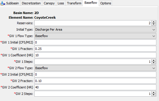
Typically, I like to use two linear reservoir layers. I use groundwater layer 1 to represent interflow, which has response times 2-5 times longer than surface flow. Interflow represent water that infiltrates, travels down slope in the soil, within the unsaturated zone, and then makes its way back onto the land surface. After reaching the land surface, the interflow water travels in the stream network to the subbasin outlet. The figure below shows possible flow paths for interflow. 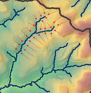
I use the groundwater layer 2 to represent groundwater flow, which has response times that are much longer than surface flow. Groundwater flow represents water that percolates to the groundwater table, the saturated zone, and then flows back onto the land surface within channels and streams. The figure below shows a possible flowpath for groundwater flow. Notice that the infiltrated water spends much longer in the soil than for interflow. 
The fraction parameter was made available starting in HEC-HMS Version 4.4 and is a way to distributed water passed to baseflow from the loss method. The summation of the fraction values, from all groundwater layers cannot exceed 1. The total fraction amount can be less than 1. For example, a groundwater 1 fraction of 0.25 and a groundwater 2 fraction of 0.1 means 25 percent of the percolation losses from the Deficit and Constant loss method is passed to the groundwater 1 layer, 10 percent of the percolation losses from the Deficit and Constant loss method is passed to the groundwater 2 layer, and 65 percent of the percolation losses from the Deficit and Constant loss method are lost to a deep aquifer and do not run off into the stream network.
The linear reservoir coefficient parameter can be used to control how quickly water is held in the groundwater layer. A small linear reservoir coefficient will result in water leaving the linear reservoir more quickly than a larger coefficient. The figure below shows results from three simulations where the linear reservoir coefficient was varied. Notice how the magnitude of the baseflow hydrograph is decreased as the coefficient is increased. A larger coefficient (for the same size watershed) means infiltrated water spends more time in the soil before flowing back onto the land surface. This example also illustrates that the linear reservoir coefficient does not have much impact on the timing of the peak flow in the baseflow hydrograph. 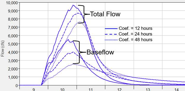
The number of steps parameter is a way to control the timing of the peak flow in the baseflow hydrograph. One step means there is one linear reservoir within the groundwater layer. Two steps means there are two linear reservoirs in series in the groundwater layer. Water is routed through one linear reservoir and then it is routed through the second linear reservoir. Each linear reservoir has the same coefficient. The figure below shows results from three simulations where the number of steps was varied. Not only is the magnitude of the baseflow hydrograph impacted by the number of steps, but the timing of the baseflow hydrograph is shifted as well. 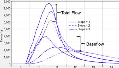
The release of HEC-HMS 4.7 provided a new a new subbasin transform method, the 2D diffusion wave transform method. The 2D diffusion wave transform method is a true cell to cell routing model, it is the same routing model (code) in HEC-RAS. After preliminary application of the 2D diffusion wave transform method to watershed scale applications, the HEC-HMS team identified the need to provide a 2D subsurface routing option that compliments the 2D diffusion wave surface routing option. This need for a integrated 2D surface-subsurface model can be illustrated using the figure below. Within HEC-HMS, baseflow from the linear reservoir baseflow method is only added to the hydrograph at the outlet of the 2D area (subbasin) and is represented by the brown dashed line in the model results shown below. Infiltrated water from all grid cells, regardless of their location in the 2D area, is routed through a linear reservoir and added to the total flow from the 2D area. We found this approach could provide adequate results at the subbasin outlet, the combination of routed surface flow and baseflow at the outlet could approximate observed flow (compare the solid blue line, computed flow, and the black line, observed flow, in the figure below). However, the 2D surface flow at interior cells would be biased low because in reality a portion of the infiltrated water does flow back onto the land surface throughout the entire watershed, not at some arbitrary location like a subbasin outlet. Notice that the simulated baseflow hydrograph adds about 20 percent of the flow magnitude to the 2D diffusion wave hydrograph at the subbasin outlet. This means that the flow/stage results for cells within the 2D mesh are lower than would be observed in this model application. It is likely that modelers will have to reduce surface roughness values within the 2D model domain to offset missing groundwater flow when calibrating a model with this type of configuration. 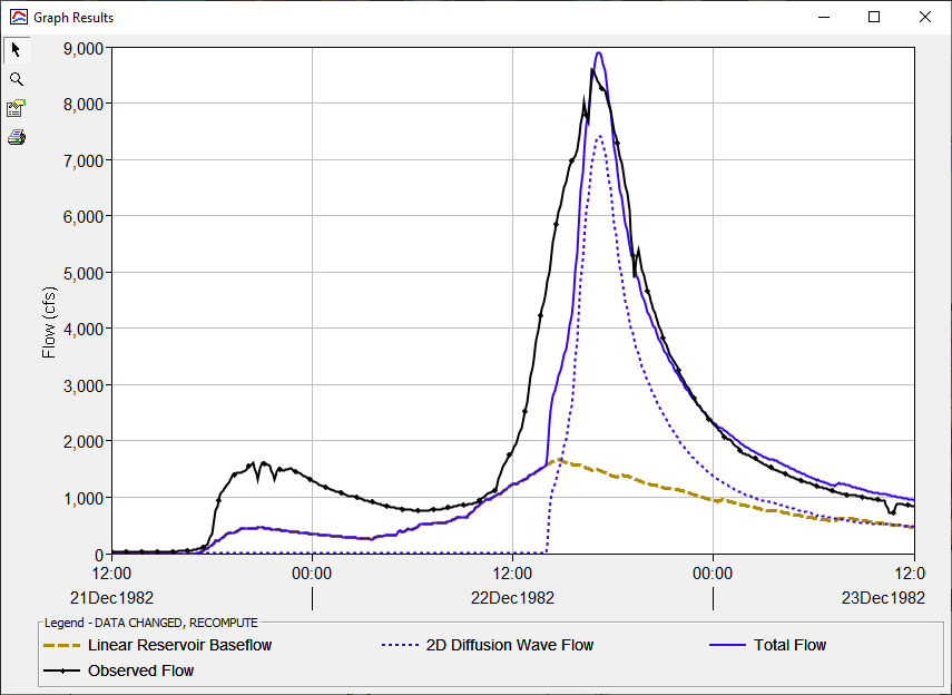
Until the HEC-HMS and HEC-RAS teams work with development partners to design and fund a true integrated 2D surface-subsurface solution, the HEC-HMS team made a modification to the linear reservoir baseflow method that allows the modeler to identify whether the Linear Reservoir groundwater layer is treated as interflow or baseflow. If the user chooses baseflow, then the routed subsurface water is added to the total flow at the subbasin outlet (outlet(s) of the 2D area). If the user chooses interflow, then the subsurface water is only routed within the 2D cell, where the infiltration happened. The routed interflow is added to the cell's surface flow and routed on the 2D surface to downstream grid cells (where it can be infiltrated again). The new interflow linear reservoir baseflow option can only be activated when the 2D Diffusion Wave transform option is selected.
It is understood this approach is conceptual and the major assumption is that all interflow leaves the cell on the surface where the infiltration happens. However, this approach does allow for improved model results for interior grid cells within the 2D area. Also, the modeler will have to adjust surface roughness values when changing to the new interflow baseflow routing option because more water will be in the channel network within the 2D area.
This tutorial shows how the new interflow option can be utilized with the 2D diffusion wave transform method, how to parameterize the linear reservoir baseflow parameters, and then shows additional model calibration that is needed when using the new interflow linear reservoir baseflow option.
Watershed Description
The area modeled in this tutorial is part of the Coyote Creek watershed in Northern California. The watershed modeled is approximately 109 square miles and is located just south and east of San Jose, CA. The location of the watershed is shown below. 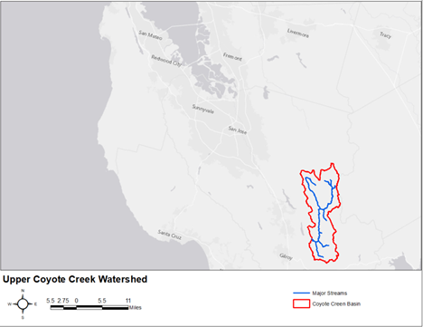
Terrain data was downloaded from the USGS National Map Viewer. The terrain data was re-projected and the vertical units were converted to feet. Published streams from the National Hydrograph Dataset (NHD) were burned into the terrain as well. The terrain data was used to delineate subbasin and stream elements within HEC-HMS. The terrain data was also used by the HEC-RAS 2D preprocessor to extract hydraulic properties for each cell and cell face in the 400-ft unstructured mesh. The following figure shows the watershed on top of an aerial image; notice the watershed is in the coastal mountains. 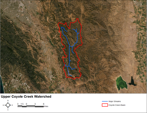
Landuse data was gathered from the National Land Cover Database (NLCD) 2016. As shown below, land uses within the watershed are mixed forest, grassland, and shrub/scrub. Soil data from the SSURGO database was used to create raster datasets of soil properties, like saturated hydraulic conductivity. The soil property datasets were used to estimate Deficit and Constant loss parameters.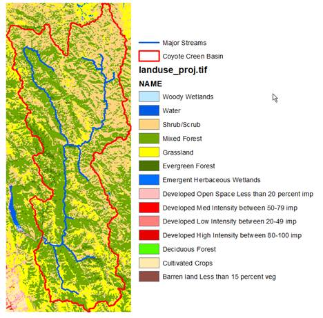
Precipitation and flow information were provided by staff at the California Department of Water Resources. Both the precipitation and flow data were recorded at 15-minute intervals. The follow figure shows the precipitation gage locations. The flow gage is located at the outlet of the watershed area. HEC-GageInterp was used to interpolate the point rain gage data to create precipitation grid sets for six storm events (a 2000-meter grid spacing was used for the interpolation). The PRISM 30-year average precipitation dataset was used as a bias grid in the interpolation process.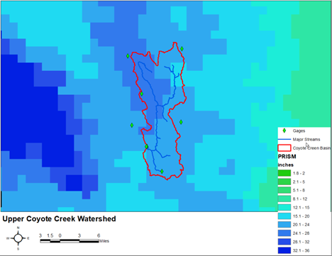
The unstructured discretization method was used to create a 2D mesh that was used with the 2D Diffusion Wave transform method. Currently, the modeler must create the 2D mesh and compute the mesh properties in HEC-RAS before referencing the mesh in HEC-HMS. A portion of a 400-ft unstructured mesh is shown on top of the Coyote Creek watershed. The unstructured mesh option can be used with gridded or lumped loss methods and with unit hydrograph, ModClark, and 2D Diffusion Wave transform methods. Gridded or non-gridded precipitation can be used with an unstructured mesh. There are 18,512 cells within the unstructured mesh.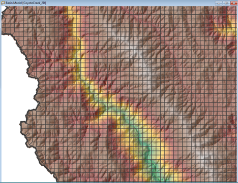
Applications of the 2D Diffusion Wave Transform and Linear Reservoir Baseflow Methods
As shown below, there are four basin models in the project linked to this tutorial. All four basin models are configured to use the Unstructured discretization, Simple Canopy, Deficit and Constant loss, 2D Diffusion Wave transform, and Linear Reservoir baseflow methods. Differences between the basin models are described below. It is important to note that only losses due to the constant loss rate within the Deficit and Constant loss method are passed to the Linear Reservoir baseflow layers. Losses due to the moisture deficit being filled are not passed to the Linear Reservoir baseflow method. 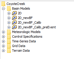
Basin Model - 2D
The 2D basin model was configured to use the "baseflow" option for both the groundwater 1 and groundwater 2 layers. This means the routed baseflow is only added to the routed surface flow at the subbasin outlet. The following table contains the constant loss rate and baseflow parameter values. The surface roughness values were adjusted as well during model calibration. This basin model is used within the 1982_2D simulation.
Constant Loss Rate (IN/HR) | 0.19 |
GW 1 Flow Type (CFS/MI2) | Baseflow |
GW 1 Fraction | 0.25 |
GW 1 Coefficient (HR) | 10 |
GW 2 Flow Type (CFS/MI2) | Baseflow |
GW 2 Fraction | 0.1 |
GW 2 Coefficient (HR) | 40 |
GW 3 Flow Type (CFS/MI2) | NA |
GW 3 Fraction | NA |
GW 3 Coefficient (HR) | NA |
The following figure shows results at the outlet of the 2D area along with the observed flow for the 1982_2D simulation. Below, the black line is the observed flow at the outlet of the subbasin and the smaller dashed blue line is the total computed flow at the outlet. The total computed flow combines surface flow, solid blue line, and baseflow, longer dashed line. Notice how the 2D surface runoff does not make it to the outlet of the 2D area until hour 1400 on December 22. If you look at the excess precipitation time series, you will see excess precipitation was computed starting at hour 1700 on December 21. Starting the simulation with a dry 2D area causes a delay in surface runoff, but the linear reservoir baseflow option masks this result by routing the infiltrated water to the subbasin outlet (baseflow is making it to the outlet before the surface runoff). Overall, the magnitude of the total flow matches well with the observed peak. However, as discussed above, if you extract results for grid cells within the 2D area, then the computed flow and stage would be biased low throughout the 2D area.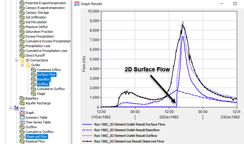
Basin Model - 2D_newBF
The 2D_newBF basin model was configured to use the new "interflow" option for both the groundwater 1 and groundwater 2 layers. The "baseflow" option was used for the groundwater 3 layer. This means a portion of the infiltrated precipitation was routed within two linear reservoir layers within each 2D cell (each layer had a different coefficient). The routed baseflow was passed to the surface model at the "outlet" of each cell.
The following table shows the constant loss rate and baseflow parameter values for this model configuration. The groundwater 1 layer had a much smaller coefficient than the groundwater 2 layer, which results in flow leaving the groundwater 1 layer more quickly than the groundwater 2 layer. Notice how the storage coefficient values are significantly smaller than the 2D basin model. The coefficients were reduced because interflow is being modeled within each 400ft grid cell, not for the entire 108.55 square mile watershed. The surface roughness values were the same as the 2D basin model. This basin model is used within the 1982_2D_newBF simulation.
Constant Loss Rate (IN/HR) | 0.19 |
GW 1 Flow Type (CFS/MI2) | Interflow |
GW 1 Fraction | 0.1 |
GW 1 Coefficient (HR) | 0.2 |
GW 2 Flow Type (CFS/MI2) | Interflow |
GW 2 Fraction | 0.1 |
GW 2 Coefficient (HR) | 10 |
GW 3 Flow Type (CFS/MI2) | Baseflow |
GW 3 Fraction | 0.1 |
GW 3 Coefficient (HR) | 20 |
The following figure shows results at the outlet of the 2D area along with the observed flow for the 1982_2D_newBF simulation. Adding the interflow baseflow output from each grid cell, along with surface runoff, and routing the surface flow to the downstream grid cells does change results significantly. The simulated peak flow is larger than in the 1982_2D simulation. This increase in magnitude is due to having more water in the channel network, and faster velocities, throughout the entire 2D area. The timing of the peak flow was 25 minutes earlier in the 1982_2D_newBF simulation than the 1982_2D simulation. The surface roughness, loss rate, and baseflow parameter would need adjustment to improve the model results (see the 2D_newbf_Calib section below).
Another note, the delay in runoff from the 2D surface model is more pronounced in this simulation since subsurface water being routed directly to the subbasin outlet is no longer masking the routing results from the surface 2D diffusion wave model.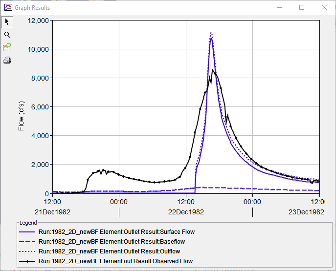 800
800
Basin Model - 2D_newBF_Calib
The 2D_newBF_Calib basin model started out as a copy of the 2D_newBF basin model. Changes were made to the surface roughness, terrain, constant loss rate, and the baseflow parameters to improve the model results. The following table shows the constant loss rate and baseflow parameter values. The surface roughness values were increased to reduce the flood magnitude. The new Terrain Reconditioning tool in HEC-HMS was used to burn in a stream network to improve conveyance (the original terrain dataset did not have channels included). The Preprocess Sinks tool was also used to remove any pits in the terrain. The modified terrain was used in the HEC-RAS model, along with the modified surface roughness values, to generate a new unstructured grid file, which was imported into the HEC-HMS project. This basin model is used within the 1982_2D_newBF_Calib simulation.
Constant Loss Rate (IN/HR) | 0.195 |
GW 1 Flow Type (CFS/MI2) | Interflow |
GW 1 Fraction | 0.1 |
GW 1 Coefficient (HR) | 0.2 |
GW 2 Flow Type (CFS/MI2) | Interflow |
GW 2 Fraction | 0.1 |
GW 2 Coefficient (HR) | 2 |
GW 3 Flow Type (CFS/MI2) | Baseflow |
GW 3 Fraction | 0.1 |
GW 3 Coefficient (HR) | 20 |
The following figure shows results at the outlet of the 2D area along with the observed flow for the 1982_2D_newBF_Calib simulation. Calibrating the model does result in a better fit to the peak flow, the time of the peak flow is slightly lagged, due to larger surface roughness values. The more important point with results from this simulation is that output from 2D surface flow better represents observations at the subbasin outlet. There is some integration of surface flow and the interflow component of subsurface flow occurring throughout the 2D area. Therefore, flow and stage at interior locations will be more accurate than the original simulation where all subsurface flow was added to surface runoff at the outlet of the subbasin. If you only need results at the outlet of the 2D area, then utilizing the interflow linear reservoir baseflow option might not provide a benefit.
The delay in surface runoff is still pronounced in this simulation. The following section shows a method for improving runoff at the beginning of the storm event. 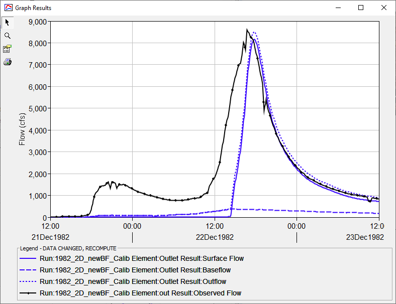
Basin Model - 2D_newBF_Calib_preEvent
The 2D_newBF_Calib_preEvent basin model started out as a copy of the 2D_newBF_Calib basin model. Changes were only made to the constant loss rate, and "fake" precipitation was added at the beginning of the simulation time window. The following table shows the constant loss rate and baseflow parameter values. The surface roughness values were the same as the 2D_newBF_Calib basin model. This basin model is used within the 1982_2D_newBF_Calib_preEvent simulation.
As shown in the figure below, the time window for the 1982_2D_newBF_Calib_preEvent simulation was extended to include precipitation occurring approximately 12 hours prior to the actual precipitation on December 21 and 22. This pre event was used to initialize the 2D area so that a small amount of water was already on the surface when the actual flood event occurred. Therefore, precipitation from the actual event being model would not be lost to natural storage in the stream network.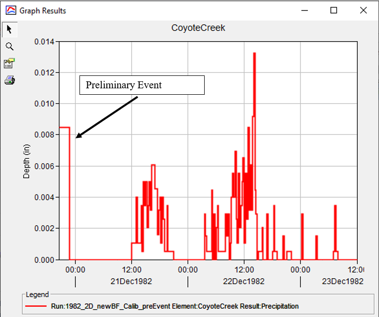
Constant Loss Rate (IN/HR) | 0.258 |
GW 1 Flow Type (CFS/MI2) | Interflow |
GW 1 Fraction | 0.1 |
GW 1 Coefficient (HR) | 0.05 |
GW 2 Flow Type (CFS/MI2) | Interflow |
GW 2 Fraction | 0.1 |
GW 2 Coefficient (HR) | 2 |
GW 3 Flow Type (CFS/MI2) | Baseflow |
GW 3 Fraction | 0.1 |
GW 3 Coefficient (HR) | 20 |
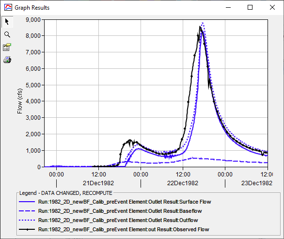
The following figure shows results at the outlet of the 2D area along with the observed flow for the 1982_2D_newBF_Calib_preEvent simulation. All basin model parameters were kept the same as the 2D_newBF_calib basin model except the constant loss rate was increased to 0.258 inches per hour. Adding a warmup period that included artificial precipitation filled streams and channels in the 2D area so that the surface response to the actual rainfall on December 21 and 22 was more realistic.