Importing and Using Parameter-elevation Regressions on Independent Slopes Model (PRISM) Precipitation Data

Introduction

This tutorial demonstrates how Parameter-elevation Regressions on Independent Slopes Model (PRISM) gridded precipitation can be obtained, imported, and used within HEC-HMS.  This tutorial will also show how simulated runoff changes when different data is used in an existing model of the Cannon River watershed. 

Download initial project files here:

• Initial HEC-HMS project
• Subbasin outline/clipping data source
• PRISM files

Note that files are provided in a compressed folder and must be unzipped.

Downloading Data

The PRISM climate group gathers climate observations from a wide range of monitoring networks and applies sophisticated quality control measures to develop gridded climate datasets.  PRISM data is collected using a horizontal resolution of 800 meters and is provided to users at a resolution of 4 kilometers.  Datasets are available in ASCII (“.asc”) or BIL (“.bil”) format.  Data is available from 1981 to present for most PRISM products including 30-year normals, daily, and monthly records. Daily PRISM data was downloaded for this tutorial.  More information about PRISM climate data can be found at the PRISM Climate Data website.

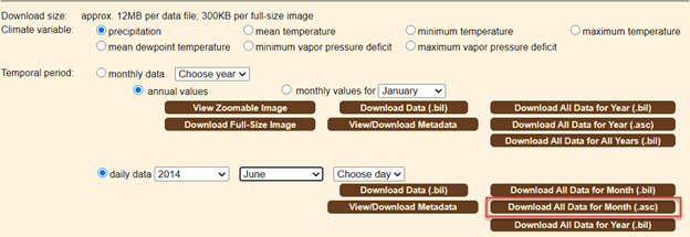
Data can be downloaded directly from the PRISM website under the “Recent Years” tab.  In this example the HEC-HMS simulation encompassed June and July of 2014, so daily data for both months was downloaded, as shown in Figure 1.  The “.asc” data was provided in a compressed file which must be unzipped prior to importing to  HEC-HMS.  The unzipped file contains the “.asc” files and projection files.

A Note on Data Quality

The quality of gridded data will vary and should be assessed to ensure the information is suitable for the purpose of the model it is being applied to.  Factors such as radar beam blockage and the distance from the radar station to the storm can affect the measurement of precipitation data.  It is recommended that gridded data be compared to other data sources to determine if it is sufficient for use in a hydrologic model.  For example, gridded precipitation can be compared to point gage data to check the magnitude and timing of a rain event.  Programs like the HEC Meteorological Visualization Utility Engine (MetVue) make is easy to compare gridded data to point rainfall.

Using the HEC-HMS Gridded Data Import Wizard

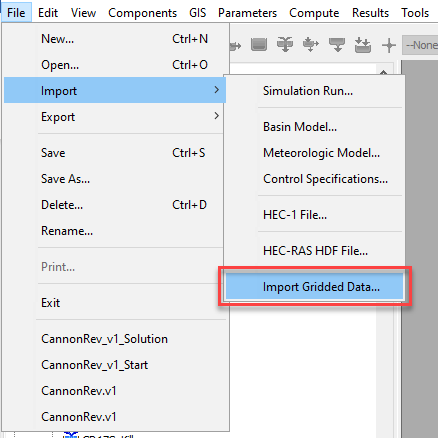
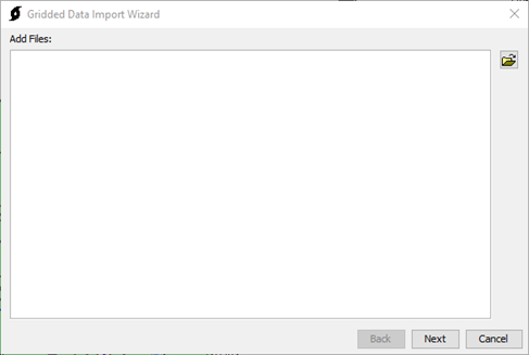
HEC-HMS can ingest multiple gridded data formats including NetCDF, HDF, GRIB, ASCII, and others.  The Gridded Data Import Wizard in HEC-HMS guides the user through importing raw gridded precipitation data and creates a DSS file which can be used to perform simulations.  The “File | Import | Import Gridded Data…” option was selected, as shown in Figure 2, to launch the Gridded Data Import Wizard, as shown in Figure 3.

Select Data Files

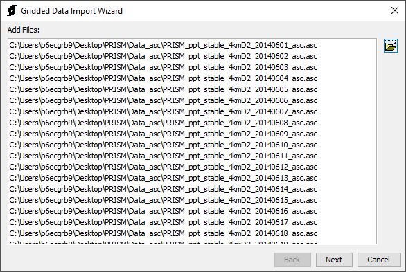
On the first panel, click the folder icon, navigate to the PRISM ASC files, select all the files (Control + A), and click “Open” to add the files, as shown in Figure 4. 

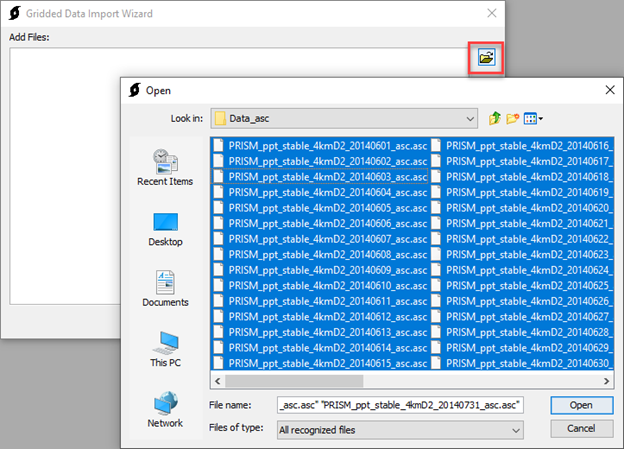
Once the raw ASC files are added, click “Next” to confirm the selection of the files, as shown in Figure 5.

Select Variables to Import

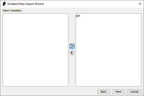
Most scientific data formats have an internal self-describing structure that organizes the data.  This includes variables, dates, extents, units, etc.  In this example, the variable “ppt”, which represents hourly total precipitation, was selected by double clicking (or using the arrow), as shown in Figure 6.  The “Next” button was clicked to finalize the selection.

Clipping Extents and Resampling Parameters

The PRISM data downloaded from the PRISM website covers the entire continental United States, which is significantly larger than the watershed of interest.  In order to reduce the size of the resultant data set, the raw data was clipped using a shapefile of the watershed.  The shapefile used to clip the data source represents the subbasin shapefile from the watershed model. 

Alternatively, the clipping shapefile can be created in HMS by selecting “GIS | Export Georeferenced Elements” and using the subbasin element type.  Be sure to buffer any polygon used for clipping by 1 to 2 miles.

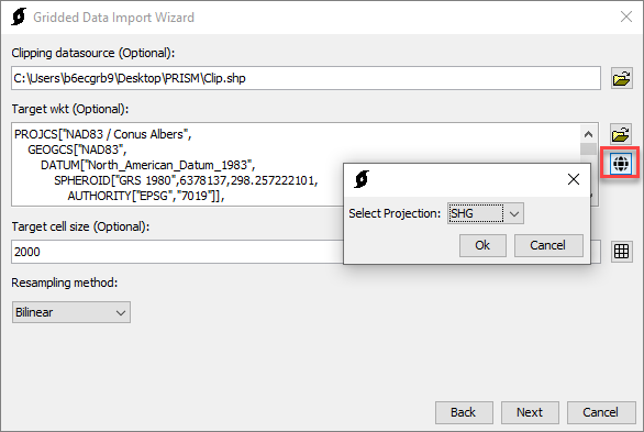
The target wkt is a coordinate reference system (CRS) in well-known text (WKT) format. The globe button can be used to select a typical CRS.  Alternatively, a PRJ projection file from a shapefile can be used. The CRS of the Standard Hydrologic Grid (SHG) was selected, as shown in Figure 7.

If the discretization is a file-specified “.mod” file, the gridded boundary conditions have to be the same cell size and projection that was used to generate the “.mod” file.  “.mod” files were commonly used within HEC-HMS models prior to version 4.7 that used gridded data.  “.mod” files in earlier versions of HEC-HMS were typically generated using the Standard Hydrologic Grid (SHG) with a 2,000 meter cell size.

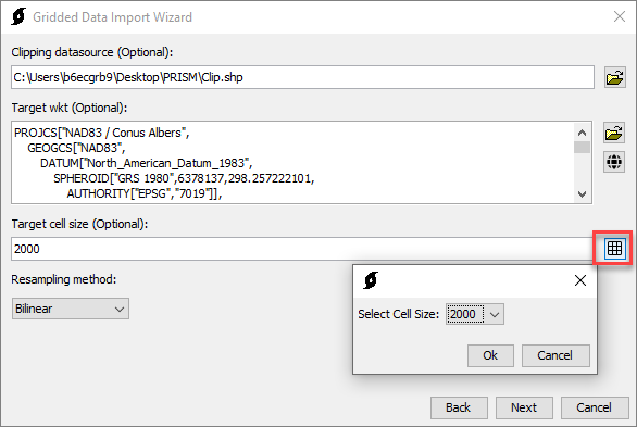
The target cell size is the cell size of the resampled grids.  It is recommended the target cell size be similar to the cell size used by the PRISM precipitation data.  In this particular case, the HMS model was developed in HEC-HMS version 4.2.1 and upgraded to version 4.7.1.  The discretization was a file-specified “.mod” file so the projection and cell size must match the projection and cell size used to create the “.mod” file.  The original modeling effort used the SHG projection with a 2,000 meter cell size.  A target cell size of 2,000 meters was selected because this is the cell size associated with the SHG, as shown in Figure 8.

Alternatively, HEC-HMS versions 4.7 and newer have the ability to update the discretization used in the model.  The model could be updated to use a structured discretization which would allow the user to alter the grid cell size and projection instead of relying on the grid cell size and projection used to create the original “.mod” file.

The resampling method is used to resample the grid to a user specified size.  The Import Wizard allows the user to select between the Nearest Neighbor, Average, and Bilinear method.  A description of each method is included below.  Select the bilinear resampling method for continuous data like precipitation.  Click “Next” once the clipping source, CRS, cell size, and resampling method are selected.

• Nearest Neighbor – A resampling technique for discrete (categorical) data which does not alter the value of the input cells.  This sampling technique is used for nominal or ordinal data where each value represents a class, member, or classification.  Examples of this type of data include land-use, soil, or forest type (ESRI, 2021).
• Average – The value of the output cell is computed from the values of all input cells which overlap the output cell (ESRI, 2021).
• Bilinear – Bilinear interpolation uses the value of the four nearest input cell centers to determine the value for the output raster cell.  The value of the output raster cell is a weighted average of these four values based on their distance from the center of the output cell.  This resampling technique is well suited for continuous data or surfaces, like temperature or precipitation (ESRI, 2021).

For HEC-HMS meteorologic models that use gridded boundary conditions, all grids should be resampled to the same CRS, extent, and grid cell size.

Destination HEC-DSS File

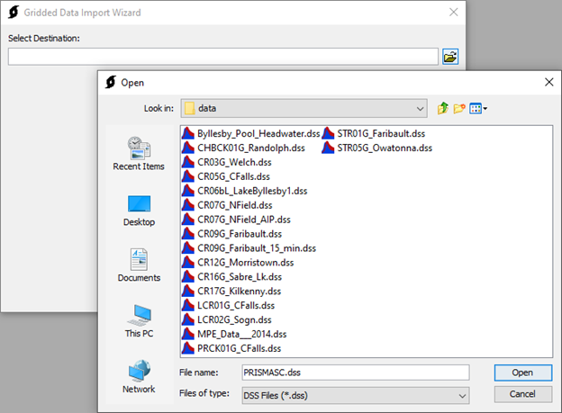
The Gridded Data Import Wizard will now import the raw gridded PRISM data and convert it to a DSS file format.  The last step is to select a destination of the DSS file that will store the gridded data.  Navigate to a directory to store the data, provide a file name with a “.dss” extension, and click “Open”, as shown in Figure 9.

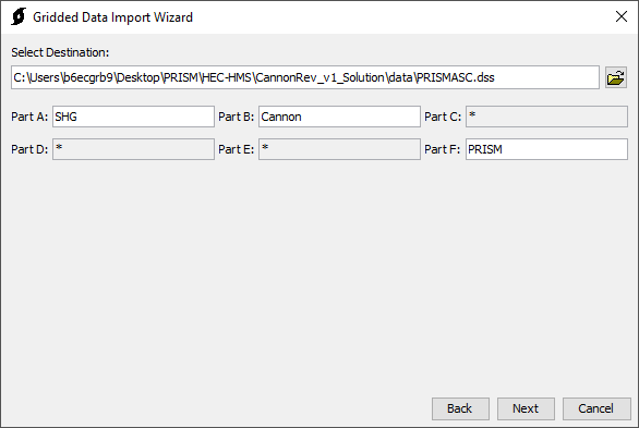
The Gridded Data Import Wizard will now allow the pathnames of the data to be defined.  Note that the C-, D-, and E-Parts of the pathnames use the wildcard asterisk because the program automatically names these parts based on the type and timestep of the data.  The user can specify the A-, B-, and F-Parts which represent the grid type, geographic area, and data source, respectively.  An example for this study is shown in Figure 10 for the Cannon River watershed study area.  Click “Next” to run the Import Wizard which creates the DSS file and converts the PRISM “.asc” data to DSS file format for use in HEC-HMS.  The time to complete this process varies depending on the amount of data but typically takes less than one minute. 

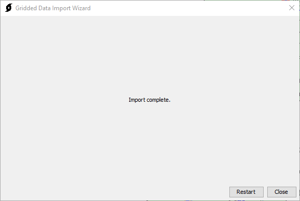
The Gridded Data Wizard will indicate when it has finished importing the data, as shown in Figure 11.  After the import is complete, click “Close” to exit the Gridded Data Import Wizard.

Using Gridded Meteorologic Data within HEC-HMS

This demonstration uses an HEC-HMS model of the Cannon River watershed in Southeast Minnesota which was developed to support a Floodplain Management Services Program study.  The model was originally calibrated using Next Generation Radar (NEXRAD) Multi-sensor Precipitation Estimator (MPE) hourly gridded precipitation data obtained from the National Weather Service North Central River Forecast Center (NCRFC).  The new PRISM precipitation grids use a daily timestep and will replace the NCRFC MPE grids.  This will illustrate how the results change when different data sources are used in the model.  Model parameters are held constant with the exception of the newly imported PRISM precipitation data.

Create New Grid Data Object

A parameter grid must be created to store the grid data.  Within HMS, select “Components | Create Component | Grid Data…” to generate a parameter grid.  Provide a recognizable name and a description of what the data represents.  The data type should be “Precipitation Gridsets”.  Click “Create” to add the new precipitation grid to the HMS model, as shown in Figure 12.

Select Previously Created HEC-DSS File and Part Names

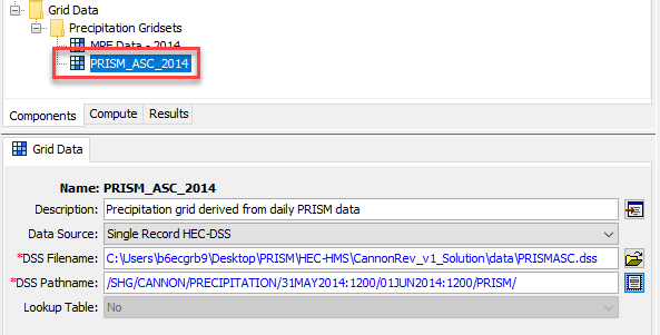
The Grid Data Object created in the previous step is now available within the “Grid Data | Precipitation Gridsets” tree in HMS.  Select the “PRISM_ASC_2014” grid created in the previous step.  The data source should be set to “Single Record HEC-DSS”.  The DSS Filename should be the pathname of the “PRISMASC.dss” file and a single pathname from the DSS file needs to be selected, as shown in Figure 13.  Any pathname within the DSS file can be selected here.

Configure Meteorologic Model

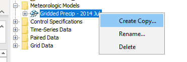
For this example, a copy of the existing “Gridded Precip – 2014 Jul” meteorological model was created by right clicking and selecting “Create Copy…”, as shown in Figure 14.  Provide a name and description for the new meteorological model.  Click “Create” when finished entering a name and description, as shown in Figure 15.  Copying the existing meteorologic model also copies the existing evapotranspiration data from the original simulation.

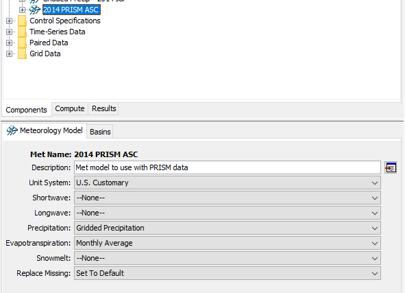
Select the “2014 PRISM ASC” meteorologic model from the Meteorologic Models tree.  Select the “Gridded Precipitation” option within the Precipitation drop down menu and set the Replace Missing option to “Set to Default”; this allows the simulation to continue if a timestep with missing data is encountered, as shown in Figure 16.

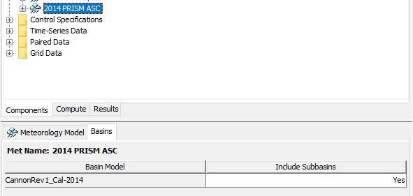
Click the “Basins” tab of the “2014 PRISM ASC” Meteorological Model and ensure that the basin model that will be used for a simulation is set to “Yes”.  In this case the basin model used is the “CannonRev1_Cal-2014” model, as shown in Figure 17.

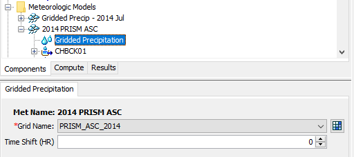
Within the “2014 PRISM ASC” Meteorological Model, highlight the “Gridded Precipitation” icon.  Select the “PRISM_ASC_2014” option within the Grid Name drop down menu, as shown in Figure 18.

Create a Simulation Run

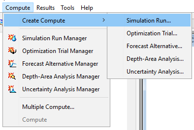
Setup a simulation run which uses the PRISM data grid, a basin model, a meteorological model, and control specifications.  For this exercise, the existing 2014 basin model and control specifications will be used rather than creating separate model components.  “Select Compute | Create Compute | Simulation Run…” to access the Create a Simulation Run Wizard, as shown in Figure 19.

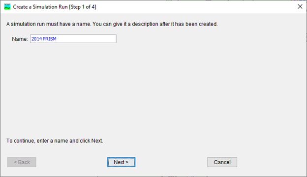
Provide a descriptive name for the simulation run, as shown in Figure 20.  Click “Next”.

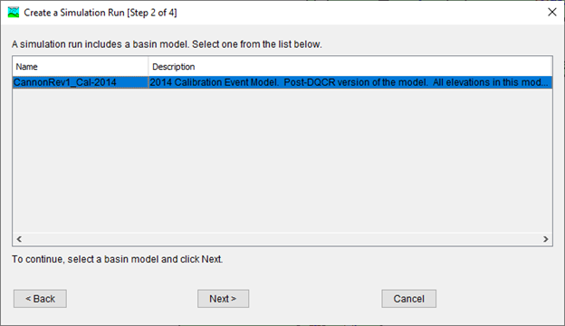
Select a basin model to use with the simulation run.  In this case, the calibrated basin model for the 2014 event (“CannonRev1_Cal-2014”) is selected for an easy comparison to show how different precipitation sources affect the results, as shown in Figure 21.  Click “Next”.

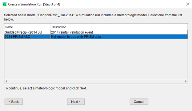
Select the meteorological model which uses the 2014 PRISM data, as shown in Figure 22.  Click “Next”.

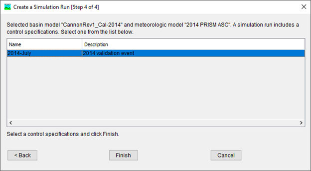
The final step is to select the Control Specifications.  For this case, the existing “2014-July” Control Specifications were used for this simulation, as shown in Figure 23.  Click “Finish”.  The simulation run is now created and ready to use.

Compute the Simulation

Select the Simulation Run that was just created from the Simulation Run drop down box, as shown in Figure 24.  Press the compute button to perform a simulation.  In this example, the simulation computed in less than 10 seconds.

Visualize Results

Visualize results by right clicking on an element of interest and selecting “View Results | Graph”.  Results from the “2014PRISM” simulation are shown in Figure 25 while Figure 26 shows the results obtain when using the original NCRFC MPE hourly precipitation data.  As the graphs show, there is a considerable difference in peak flow when different data sources are used.  All model parameters were held constant and the only difference between the two scenarios is the source of the precipitation data.

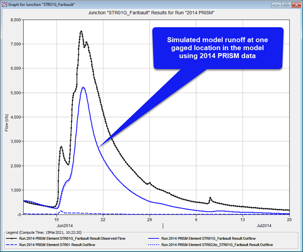
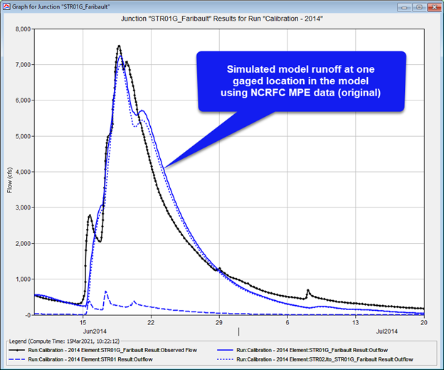
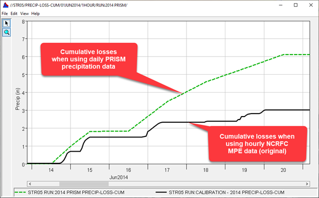
The “STR05” subbasin in the model was selected to evaluate how precipitation and loss differs when daily PRISM data is used instead of hourly NCRFC MPE data.  The two factors which influence the difference in the runoff response the most are the amount of total precipitation and how losses are computed in the model.  Table 1 shows that the PRISM data resulted in more total precipitation but also resulted in significantly more loss and less direct runoff.

Table 1. STR05 Subbasin Precipitation and Loss Summary

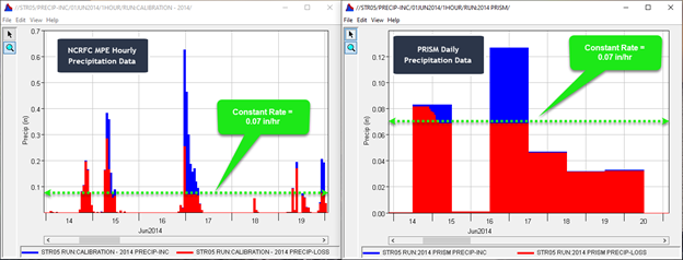
Figure 27 compares results from using NCRFC hourly precipitation data (on the left) to PRISM daily precipitation data (on the right) for the “STR05” subbasin in the model.  The blue bar in each graph represents precipitation and the red bar represents loss.  The original model simulation time step was setup and calibrated using an hourly time step.  The constant loss rate estimated for the “STR05” subbasin was 0.07 inches per hour.  In the example below, the PRISM dataset is a daily dataset that HMS automatically converts to hourly values to match the HMS simulation time step.  Representing the daily total precipitation in even hourly increments results in the incremental precipitation PRISM data rarely exceeding the constant loss rate of 0.07 inches per hour.  Runoff occurs in HMS when the precipitation rate exceeds the infiltration rate.  When NCRFC MPE hourly precipitation data is used, there are many timesteps where the precipitation rate is significantly greater than the constant loss rate and and has a higher intensity than the PRISM data.

Cumulative losses for the original analysis using hourly NCRFC MPE data are compared against cumulative losses using daily PRISM precipitation data in Figure 28.  The image shows that the PRISM version of the model results in higher losses because the hourly representation of daily PRISM precipitation data in HMS for this model is rarely intense enough to overcome the constant loss rate resulting in more loss.

The purpose of this tutorial is to show how alternate precipitation data sources can be imported into HEC-HMS using the Gridded Data Import Wizard.  Daily PRISM precipitation data was successfully imported and used to perform a rainfall runoff simulation in HEC-HMS.  This tutorial also highlights the importance of selecting an appropriate dataset for the watershed.  In this case, the Cannon River watershed is relatively small and using hourly NCRFC MPE precipitation data is beneficial to accurately capture the rainfall runoff response and losses.

Download final project files here: Final HEC-HMS project

Note that files are provided in a compressed folder and must be unzipped.

Useful Links

PRISM Data - Oregon State University

ABRFC - Sources of Error in Gridded Precipitation Measurements

References

ESRI. (2021). ArcGIS Desktop. Retrieved from Cell size and resampling in analysis: https://desktop.arcgis.com/en/arcmap/latest/extensions/spatial-analyst/performing-analysis/cell-size-and-resampling-in-analysis.htm

PRISM Climate Data. (2021). Retrieved from PRISM Climate Group, Oregon State University: https://prism.oregonstate.edu/