Download PDF
Download page Additional Questions for Applying Simplex Optimization.
Additional Questions for Applying Simplex Optimization
Last Modified: 2024-05-29 06:15:09.17
These questions were developed for the Applying the Simplex Optimization Search Method for Single Event Calibration workshop as part the Advanced Applications of HEC-HMS class.
You can use your model developed in the previous steps or download the final project files from the Introduction to Applying the Simplex Optimization Search Method for Single Event Calibration.
Project Files
Questions
Switch to the Results tab of the Watershed Explorer and examine the various results for the Opt Apr 1994 trial.
Discussion Question 1: What is the difference in peak flow between the computed and observed hydrographs? What is the time difference in peak flow?
Information about the volume, peak flow, time of peak flow, and time of center of mass is given in the Objective Function Summary table. You can view the table by going to the Results tab in the Watershed Explorer and clicking on the Objective Function Summary node under an Optimization Trial node. Your results should be similar to those shown in figure below.

Discussion Question 2: What parts of the hydrograph match the observed data well? Which parts do not match?
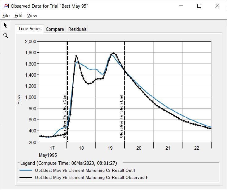
You could start by simply looking at the time-series graph. Go to the Results tab on the Watershed Explorer and click on the Optimization Trial. Choose the Observed Data graph. The first tab is the time-series graph and is shown below. Inspection of the figure shows that the initial period of baseflow recession, before the event begins, matches the observed data somewhat poorly. The rising limb of the hydrograph is a pretty good match, however.

Other graphs can also help us to see where the match is good and where it is poor. The Compare graph (second tab) and the Residuals graph (third tab) shown below can help. The Compare graph plots the computed flows against the observed flows. The one-to-one (45 degree) line indicate a perfect fit between simulated and observed data. You can see that the values fall around the 45 degree line but in general are higher or lower than it. While there may be a linear relationship between the computed and observed flow after the peak, the points do not fall on a 45 degree line.

The residuals in the figure below are computed by subtracting the observed flow from the computed flow. Negative residuals indicate computed flow is too low, while positive residuals indicate computed flow is too high. Ideally, the residuals would have a mean of zero and small variance. You can see in the figure below that the residuals swing back and forth about zero, which is consistent with the spread around the 45 degree line on the comparison graph (zero residual would fall directly on that 45 degree line).

Make at least three additional trials using the same simulation run. Adjust parameter initial values, constraints, the objective function time window, the objective goal and statistic, tolerance, or maximum number of iterations to see their effect on the optimization. Use Table 1 below to document each of your trials. You can download templates for the tables in the Project Files section at the top of this page.
Table 1. Trial results for the April 1994 event.
| Trial | |||||
|---|---|---|---|---|---|
| 1 | 2 | 3 | 4 | 5 | |
Name of modified setting | |||||
Value of modified setting | |||||
Final Parameter | |||||
| No. Iterations to Converge | |||||
| Objective Goal / Statistic | |||||
| Time of Concentration | |||||
| Clark Storage Coefficient | |||||
| Initial Loss | |||||
Constant Loss Rate | |||||
| Objective Function Value | |||||
| % Difference Volume | |||||
| % Difference Peak Flow | |||||
Continue to the other two Optimization Trials, Opt May 95 and Opt May 96. Experiment with convergence criteria and different objective functions. When you have found your best optimization results for each of the trials, enter your parameter values in the table. The observed peak flow is shown for each event. Based on your results and engineering judgment, select Adopted Values for the time of concentration and storage coefficient.
Inspect the settings in the optimization trials titled Best Apr 94, Best May 95 and Best May 96 in the final project file. Parameter summary and hydrograph comparison plots for the three trials are shown below.
Table 2. Best optimization results for each event and adopted values.
| Parameter | Apr 1994 (6,368 cfs) | May 1995 (1,786 cfs) | May 1996 (2,942 cfs) | Adopted value |
|---|---|---|---|---|
| Time of Concentration (hr) | 7.8 | 8.1 | 10.2 | 8 |
| Clark Storage Coefficient (hr) | 18.6 | 54.5 | 34.8 | 19 |
Initial Loss (in) | 0.03 | 0.006 | 0.47 | 0.05 |
| Constant Loss Rate (in/hr) | 0.05 | 0.017 | ~0 | 0.05 |


Discussion Question 3: If you use the adopted parameter values, do they produce acceptable results for the April 1994 event? How do they compare with the optimal parameters you calculated for the April 1994 event? What effect do the adopted parameters have on the April 1994 simulated hydrograph compared to the hydrograph produced by your best optimized parameters? What about other events?
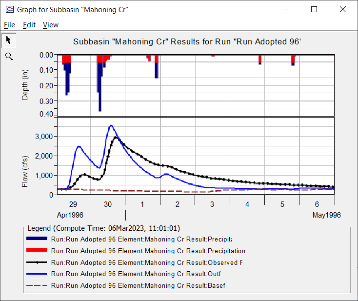
The three figures below show calibration results for the three results with the adopted values of 19 hours for the Storage Coefficient and 8 hours for the Time of Concentration. You may need to create a separate Basin Models for each run to reflect the different initial baseflow values. The fit is worse for the two smaller events. This illustrates that Clark Unit Hydrograph transform method parameters are not independent from event magnitude. The choice of calibration parameters should also be influenced by the intended use of the model. If it will be used to model flood events, the larger calibration storm is appropriate.
In addition, remember that we are trying to estimate the time of concentration and storage coefficient parameters so we want to concentrate on looking at the parts of the hydrograph that will be helpful. Where the April 1994 and May 1996 events were caused by one large burst of precipitation, the May 1995 event had two bursts of precipitation that make it difficult to discern unit hydrograph parameters.


This concludes the workshops for Applying the Simplex Optimization Search Method for Single Event Calibration.
Continue to Applying the Differential Evolution Optimization Search Method for Single Event Calibration.