Download PDF
Download page Applying the Differential Evolution Optimization Search Method for Continuous Simulation Calibration.
Applying the Differential Evolution Optimization Search Method for Continuous Simulation Calibration
HEC-HMS version 4.9 beta 6 was used to create this tutorial.
You can download a copy of the dataset here - Russian_River.zip
Introduction
This tutorial provides another example application of the Differential Evolution search method within the HEC-HMS Optimization Trial simulation type. The Single Event Optimization tutorial showed an application to a single flood event while this tutorial demonstrates application to a three year continuous simulation. The tutorial shows model performance for a simulation that used basin model parameters based on initial estimates. Then, results from manual calibration are presented. Finally, the tutorial shows results from different optimization trials that were set up using the Differential Evolution and Simplex search methods and different objective functions.
Automated optimization can be a valuable tool, but it should not replace an understanding of the software, modeling methods and assumptions, impacts from individual model parameters, and knowledge of the watershed. A modeler should not rely solely on an automated optimization tool, otherwise unrealistic parameter values or parameter combinations are possible. Understanding the runoff response for a watershed, parameter impacts, and minimum/maximum parameter ranges are required to successfully set up an optimization trial and critically evaluate results.
Example
A watershed in Northern California is used for this example. As shown in the figure below, the 92 square mile watershed was represented with one subbasin element. The Simple Canopy, Deficit and Constant Loss, Clark Unit Hydrograph Transform, and Linear Reservoir Baseflow methods were used within the Basin Model. Subbasin average precipitation and evapotranspiration were specified in the meteorologic model, both meteorologic boundary conditions were computed outside of HEC-HMS using gages located near the watershed. There is an inter-basin transfer of water from an adjacent watershed. The Potter Valley Source element was used to add the transferred water. Flow from the USGS 11461500 EF RUSSIAN R NR CALPELLA CA gage was added as observed flow to the Calpella Gage Junction element.
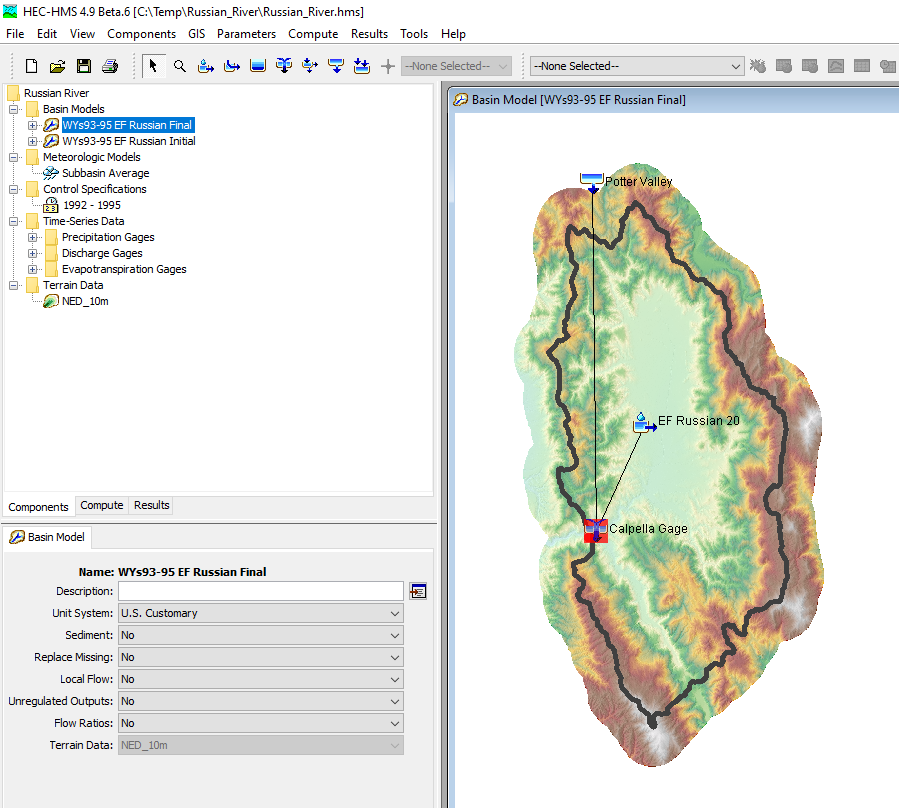
The table below contains initial parameter estimates and final parameter values after calibrating the model to observed flow data for a 3 year period, between 01Oct1992 - 01Oct1995. The initial parameter estimates were determined using GIS datasets, watershed characteristics, and knowledge gained from modeling similar watersheds in the region. Manual calibration was performed by adjusting key model parameters that improved metrics like Nash Sutcliffe and total runoff volume. Model parameters were adjusted within reasonable bounds. Also, the model was simplified by setting the GW 1 coefficient to be equal to the Clark storage coefficient and then using the GW 1 reservoirs parameter to adjust timing and shape of the interflow (GW 1) response.
Only six parameters were adjusted during manual model calibration, these six parameters are highlighted in the table below.
| Parameter | Initial Estimates | Manual Calibration |
| Maximum Canopy Storage(in) | 0.1 | 0.1 |
| Crop Coefficient | 0.7 | 0.7 |
| Initial Loss (in) | 2.5 | 2.5 |
| Maximum Deficit (in) | 6 | 6 |
| Constant Rate (in/hr) | 0.25 | 0.13 |
| Impervious (%) | 0 | 0 |
| Time of Concentration (hr) | 5 | 5.5 |
| Storage Coefficient (hr) | 8 | 4.5 |
| GW 1 Initial Flow (cfs/mi2) | 0 | 0 |
| GW 1 Fraction | 0.5 | 0.3 |
| GW 1 Coefficient (hr) | 8 | 4.5 |
| GW 1 Reservoirs | 2 | 3 |
| GW 2 Initial Flow (cfs/mi2) | 0 | 0 |
| GW 2 Fraction | 0.4 | 0.4 |
| GW 2 Coefficient (hr) | 100 | 100 |
| GW 2 Reservoirs | 1 | 1 |
Calibrating a model to a continuous precipitation-runoff record is significantly more difficult than calibrating a model to a single event. More hydrologic processes need to be included in the model, like baseflow, evaporation, and transpiration. In addition, obtaining boundary condition data that adequately describes all precipitation events is difficult. Often, there is under and over estimation of the boundary conditions from event to event within the simulation, which makes it challenging to find one parameter set that performs well. Modelers can fall into the trap of emphasizing a single event which causes the model to perform poorly for other events within the simulation time window.
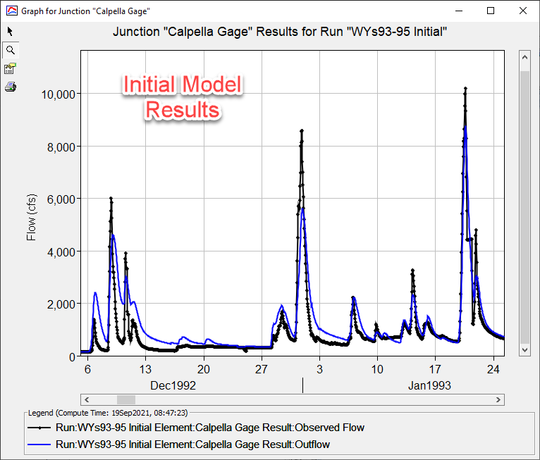
The following figures show results from both the initial simulation (uncalibrated model) and from the manually calibrated model. Notice the Nash Sutcliffe metric improved from 0.806 to 0.895 from the initial model to the manually calibrated model. The runoff volume was already within an adequate range for the initial model results.
You need to zoom into specific flood peaks when simulating a longer period of record that contains multiple flood peaks to determine whether the time of peak flow is similar to observations. Results from the initial model showed computed runoff peaking after observed flow, and generally the simulated flood peak was less than the observed flood peak. The Clark storage coefficient and GW 1 coefficient parameters were decreased to improve the shape and timing of the computed hydrograph. The constant loss rate, Clark storage coefficient, and Linear Reservoir GW 1 parameters were adjusted to improve the magnitude of the modeled runoff peaks.

The figure below shows a zoomed in portion of the initial model simulation. Notice the model's timing of the flood peaks is lagged from the observed record and the model's magnitude of peak flow is less than the observed record as well.
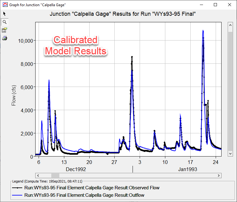
The figure below shows the same period as the figure above but includes the final, or calibrated, model results. The model's timing and magnitude are improved.
HEC-HMS Optimization Trials Comparison
Four optimization trials were configured to explore possible solutions from the automated Differential Evolution and Simplex search methods. Currently, the Optimization Trial is somewhat limited, linking parameters together is not possible, and the Linear Reservoir Fraction parameter cannot be selected. Because of the limitation with the Linear Reservoir Fraction parameter, the calibrated basin model was selected for each of the optimization trials. The calibrated basin model contained the adjusted Linear Reservoir Fraction parameter values. The Optimization Trials were configured to adjust the Constant Loss Rate, Clark Time of Concentration, Clark Storage Coefficient, Linear Reservoir GW 1 Coefficient, and Linear Reservoir GW 1 Reservoirs.
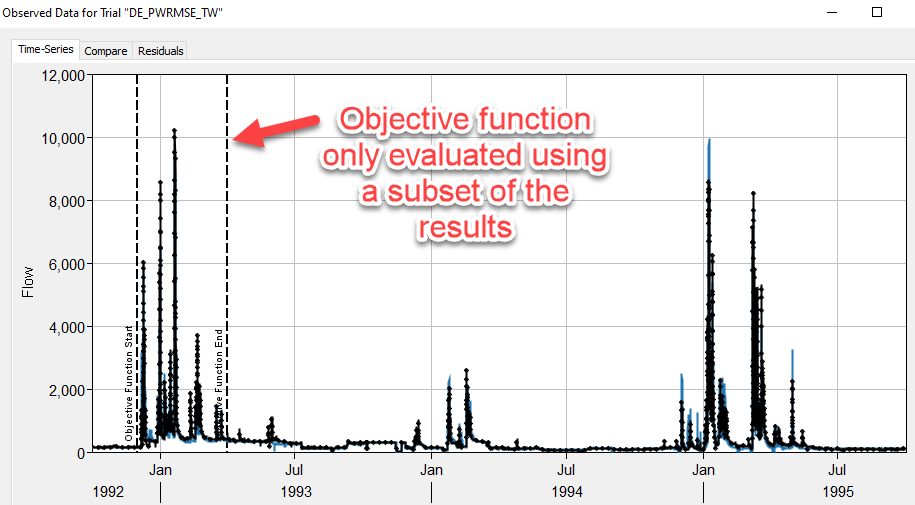
The list below shows which search method and objective function were selected for each of the optimization trials. The DE_PWRMSE_TW trial was added to explore if there was a noticeable advantage to shorten the time window used to compute the objective function. As shown in the figure below, the runoff response in Northern California is characterized by a wet winter/early spring and a dry summer/fall. Instead of computing the objective function using data for the entire simulation time window, HEC-HMS includes an option to reduce the objective function time window to emphasize a specific period.
- DE_NS - Differential Evolution Search method and the Nash Sutcliffe Objective Function
- DE_PWRMSE - Differential Evolution Search method and the Peak-Weighted Root Mean Square Error Objective Function
- DE_PWRMSE_TW - Differential Evolution Search method, Peak-Weighted Root Mean Square Error Objective Function, and a shortened window to evaluate the Objective Function (01Dec1992 to 03Apr 1993)
- Simplex_PWRMSE - Simplex Search method and the Peak-Weighted Root Mean Square Error Objective Function
Final parameter values from the optimization trials and the manual calibration are contained in the table below. The Nash Sutcliffe metric is approximately the same among the automated optimization trials and the manual calibration. However, some of the parameters have a large amount of variation between automated and manual calibration.
| Parameter | Initial Estimates | DE_NS | DE_PWRMSE | DE_PWRMSE_TW | Simplex_PWRMSE | Manual Calibration |
| Constant Rate (in/hr) | 0.25 | 0.15 | 0.14 | 0.09 | 0.13 | 0.13 |
| Time of Concentration (hr) | 5 | 3.41 | 3.04 | 3.21 | 3.00 | 5.5 |
| Storage Coefficient (hr) | 8 | 6.79 | 9.62 | 13.47 | 10.15 | 4.5 |
| GW 1 Coefficient (hr) | 8 | 4.01 | 3.00 | 3.0 | 3.41 | 4.5 |
| GW 1 Reservoirs | 2 | 2 | 2 | 2 | 2 | 3 |
| Nash Sutcliffe | 0.81 | 0.91 | 0.91 | 0.89 | 0.91 | 0.90 |
The final/optimal Clark time of concentration value within the Simplex_PWRMSE optimization trial converged to the minimum value (3 hours was the minimum and 25 hours was the maximum). A time of concentration of 3 hours is generally too short for a watershed of 92 square miles. Based on the longest flowpath length for this watershed, an average velocity of 8 ft/s is computed using a time of concentration of 3 hours. The automated optimization trial offset the low Clark time of concentration value with a high Clark storage coefficient value.
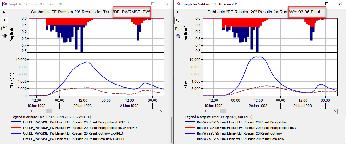
Conceptually, the GW 1 Coefficient and Reservoir parameters should produce a baseflow hydrograph that peaks after the unit hydrograph's response (direct runoff or overland flow). GW 1 typically represents interflow, which includes water that infiltrates into the soil, flows down-gradient within the unsaturated zone, and then flows back onto the land surface where the water travels in the channel network to the subbasin outlet. The final GW 1 parameters from the Differential Evolution and Simplex trials that used the Peak-Weighted RMSE objective function produce groundwater hydrographs that peaked before surface runoff. The figure below shows results from the DE_PWRMSE_TW and manually calibrated model (simulation run name WYs93-95 Final). The brown dashed line is the simulated baseflow response. Notice how the baseflow response from the DE_PWRMSE_TW simulation peaks before or concurrently with direct runoff. As a rule of thumb, the GW 1 coefficient should not be smaller than the Clark storage coefficient, unless the number of GW 1 reservoirs is large.
The optimization trials could have been run a second time where the Clark storage coefficient and GW 1 coefficient values were set equal to one another and locked (when locked, the program does not vary the parameter value during the optimization trial). Then, the minimum GW 1 reservoirs parameter could have been set to 2 in order to force a baseflow response that lagged the surface runoff response.
The following table contains the run time and number of iterations for each of the Optimization Trials.
| Optimization Trial | Run Time (minutes) | Number of Evaluations |
|---|---|---|
| DE_NS_ | 37 | 20 iterations x 30 population size = 600 |
| DE_PWRMSE | 70 | 36 x 30 = 1080 |
| DE_PWRMSE_TW | 85 | 38 x 30 = 1140 |
| Simplex_PWRMSE | 18 | 163 |
Summary
The automated optimization tools can be used to find parameter sets for both single events and continuous simulation; however, it is important to critically evaluate results from the automated optimization. The modeler must make sure parameter values are reasonable. As shown in this tutorial, use of the Optimization Trial should be an iterative process. Initially, the minimum and maximum parameter ranges should be set to guarantee reasonable parameter values are identified as part of the optimization. Due to interactions between parameters (the constant loss rate, Clark storage coefficient, and Linear Reservoir GW 1 parameters can significantly impact the magnitude of the modeled runoff peak flow), reducing the number of parameters adjusted during the optimization trial can reduce the possibility of the optimization trial converging to an unrealistic parameter set.