Last Modified: 2025-04-09 09:25:18.262

Software Version

An unofficial version of HEC-HMS version 4.13 (not publicly available) was used to create this tutorial. It should not be used other than for testing the new Optimization Trial enhancements.

For now, you may download an unofficial portable build here: https://drive.hecdev.net/share/X8ufbMKQ

Project Files

Download the initial HEC-HMS project files here:

NAB_West_Branch_Susquehanna_Initial.zip

Overview

As a result of CWMS funding to add forecast optimization features to HEC-HMS, the stand-alone Optimized Trial simulation type in HEC-HMS has benefitted from several key enhancements which have expanded on its utility and areas of application. Examples of the Optimization Trial enhancements are outlined below. This tutorial and guide along with the associated project files will help you explore the new optimization enhancements and functionality.

Multiple Objective Functions

In previous versions of HEC-HMS, the Optimization Trial was limited to a single objective function which meant that only one location and one time-window could be optimized for at a given time. Starting in version 4.14, HEC-HMS now allows for multiple objective functions to be specified within an Optimization Trial, meaning that multiple locations and/or multiple time-windows can now be leveraged within an optimization routine. As an example, if you were calibrating a model to a multi-peaked rainfall-runoff event at a location of interest, you could specify multiple objective functions each at the target location but each with unique time-windows that capture the multiple peaks. An optimization routine could then find the singular parameter set that best matches the multiple, observed peaks.

Multi-Time Window Optimization

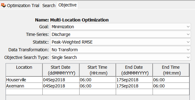
As a second example, if you wanted to find a singular parameter set that best matches observed streamflow data at two separate locations, a singular optimization routine can now be set up that accounts for both observed data in its search. When multiple objective functions are specified in a singular optimization routine (using "Single Search"), each of the objective function results are combined via addition and assessed cumulatively.

Multi-Window Optimization

Sequential Searches

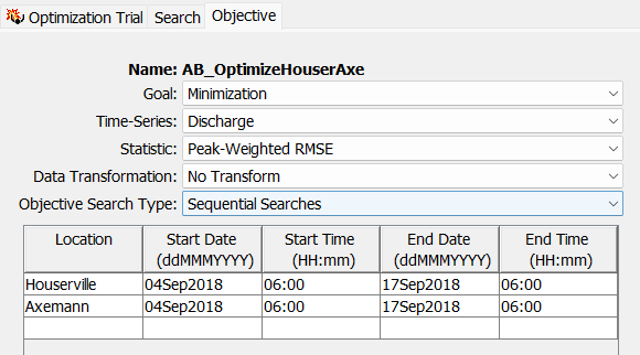
Starting in version 4.14, an Optimization Trial now allows for iterative "Sequential Searches". If this option is selected, a separate optimization routine will be computed for each target location starting upstream and progressing downstream. For example, once an optimized parameter set for the most upstream target location is found, those parameter values will be locked into place and used for the subsequent optimization search routine that occurs at the next target location downstream. If "Single Search" is selected, only one optimization routine will be computed with the objective function value at each target location being added (as described in the above section).

Sequential Searches

Sequential Search

The Sequential Searches option is only available if the selected optimization goal is minimization and there are multiple, unique target locations selected.

Sequential Search

The Sequential Searches option is currently only available for a Simplex search. Furthermore, Sequential Searches is only allowed for Optimization Trials that contain element-based or subbasin zone-based optimization parameters.

New Optimization Parameter Type - Subbasin Zone

Previous versions of HEC-HMS allowed for several different categories of Optimization Parameters including element-based method parameters, precipitation parameters, and "All-Subbasin" scale-factors. Starting in version 4.14, a new "Subbasin Zone" scale-factor parameter type was created. If the basin model associated with an Optimization Trial has at least one Zone Configuration with Zone regions previously created, the "Subbasin Zone" Optimization Parameter type is accessible. This allows the optimization routine to find a scale-factor parameter set based on all of the subbasins within a specified Zone.

Optimization Parameter - Subbasin Zone

Background

The project files in this tutorial and guide model Bald Eagle Creek (a tributary of the West Branch Susquehanna River) and the drainage area above Foster Joseph Sayers Dam (339 square miles). Foster Joseph Sayers Dam is located approximately one mile upstream from Blanchard, PA and 14 miles above the mouth at Lock Haven, Centre County, PA. The dam is an earth fill construction with a maximum height of 100 feet above the streambed and a top length of 6,835 feet. It has a gated outlet tunnel for the regulation of flood flows. The spillway, located in rock in a saddle adjacent to the left abutment, is uncontrolled. The reservoir has a storage capacity of 99,000 acre-feet at spillway crest and a drainage area of 339 square miles. The project was completed in 1969.

Bald Eagle Creek Watershed

Multiple Objective Functions - Time Windows

Download the "NAB_West_Branch_Susquehanna.zip" file to your C drive and extract it.
Open HEC-HMS version 4.14 or newer.
Click File | Open and navigate to the "NAB_West_Branch_Susquehanna.hms" file within the extracted folder to open the project.
In the Watershed explorer, click the Compute tab and then expand the Optimization Trials node.
Select the Optimization Trial named "A_OptimizeHouserville" which has an optimization routine already setup for the most upstream portion of the watershed.
As seen in the below figure, the Objective tab shows that one objective function has been setup with a location of Houserville and a time-window that encompasses the entire simulation period. A minimization goal has been set using Peak-Weighted RMSE to reach a solution that best matches the observed discharge time-series data at the Houserville location.
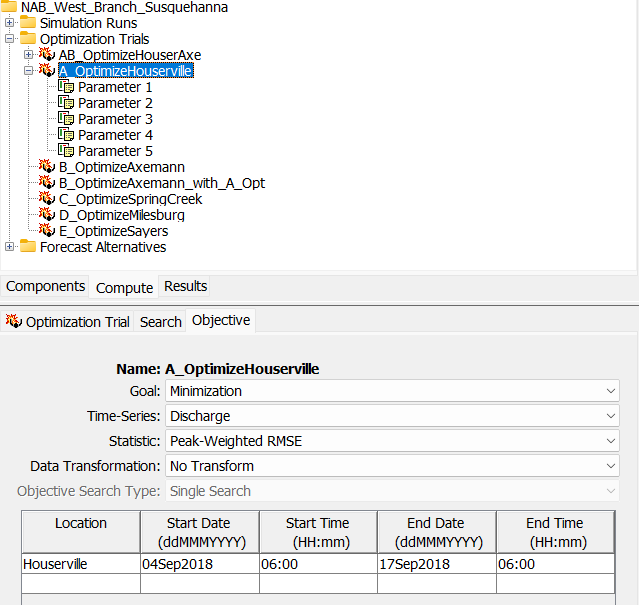
In this case, the only upstream element in the basin model is the "Spring_Crk_ab_Houser" subbasin. Five element-based optimization parameters have been configured for the subbasin, including two optimization parameters related to Deficit and Constant loss method parameters and three related to Recession baseflow method parameters.

Parameter Bounds

To achieve the best optimization results, it is important to define realistic minimum and maximum bounds for each optimization parameter.
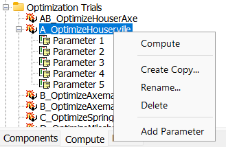
Compute the "A_OptimizeHouserville" optimization trial via the right-click option. The optimization trial should converge on a solution after roughly 130 iterations.
Navigate to the Results tab, expand the Optimization Trials node, and select the "A_OptimizeHouserville" optimization trial. Select the Optimized Parameters table. Also, expand the Houserville folder and select the Observed Data plot. The five optimized parameter values (albeit Parameter 3 was set to "locked" in this example) led to a good visual match between the computed and observed time-series data.
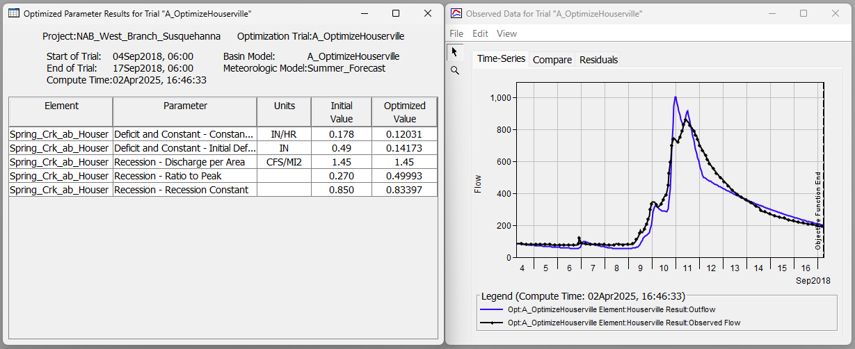
While the optimized parameters led to a good fit of the observed data across the entire simulation window, let's pretend that we were only interested in closely matching the peak of the hydrograph and the recession limb. We can define multiple objective function time windows to achieve this outcome
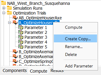
Create a copy of the "A_OptimizeHouserville" optimization trial by navigating to the Compute tab, right-clicking the A_OptimizeHouserville node, and selecting Create copy. Name the copy "Multi-Window Optimization".
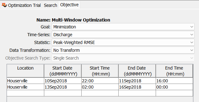
Select and expand the newly created "Multi-Window Optimization" node and navigate to the Objective tab. Let's narrow the start and end dates/times so that they encompass only the time period that the observed peak occurs. Specify the below time-window changes.
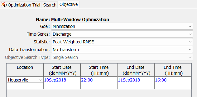
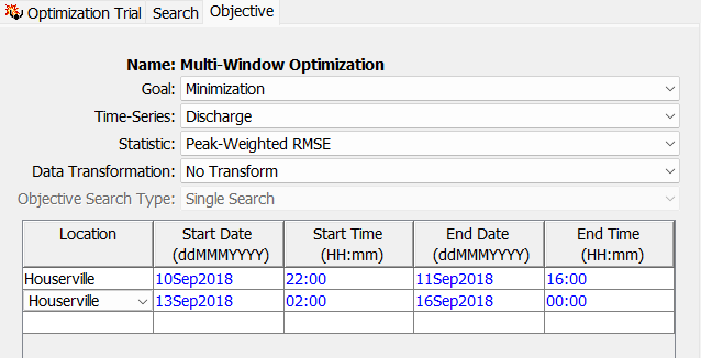
Now let's create a second objective time window by double-clicking in the first column of the next row and selecting Houserville. Let's specify stand and end dates/times so that they encompass a portion of the observed recession limb. Specify the below time-window entries for this second objective.

Multiple Time Windows

When multiple time windows are specified at the same location, they must NOT overlap.
Save your project. Compute the "Multi-Window Optimization" simulation.
After 150 iterations, the Simplex search will fail to converge. The optimization trial has a neat feature that allows you to increase the maximum iteration and then pick back up where you left off when you re-compute.
Navigate to the Search tab and increase the Max Iterations entry from 150 to 200. Save and recompute. The simulation should re-start at iteration 150 (unless you clicked force-compute or changed other parameters) and converge after roughly 180 iterations.
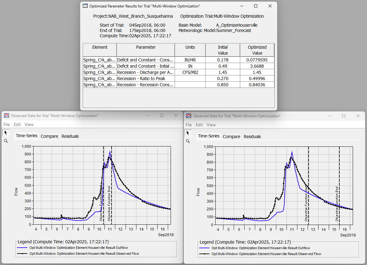
Navigate to the Results tab and expand the "Multi-Window Optimization" simulation node. Notice that there are two "Houserville" folders, one for each specified objective function. View the Optimized Parameters table and view both of the Observed Data plots contained in the two folders. The only difference in the two Observed Data plots are the vertical, dashed lines denoting the two distinct time periods that the optimization routine used in its evaluation. The optimized parameter values achieved a better fit of the observed peak and of the specified portion of the recession limb. You'll notice that the optimized values, particularly those relating to the Decifict and Constant parameters, are different than the previous optimization trial that used one objective function that covered the entire simulation period.

Multiple Objective Functions - Locations

Navigate to the Compute tab and create a copy of the "AB_OptimizeHouserAxe" optimization trial. Name the new trial "Multi-Location Optimization".
Select and expand the newly created "Multi-Location Optimization" node and navigate to the Objective tab. Notice that there are two objective functions specified, one for the Houserville location and one for the Axemann location further downstream.
For this example, let's change the Objective Search Type to Single Search. We will explore the new Sequential Searches feature later on.
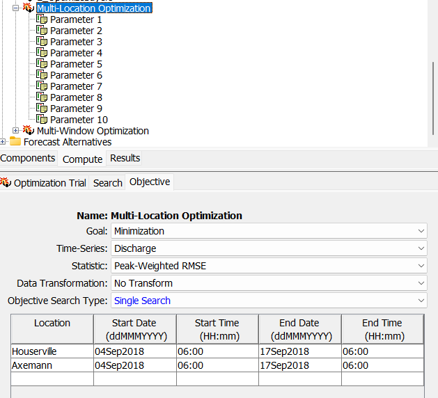
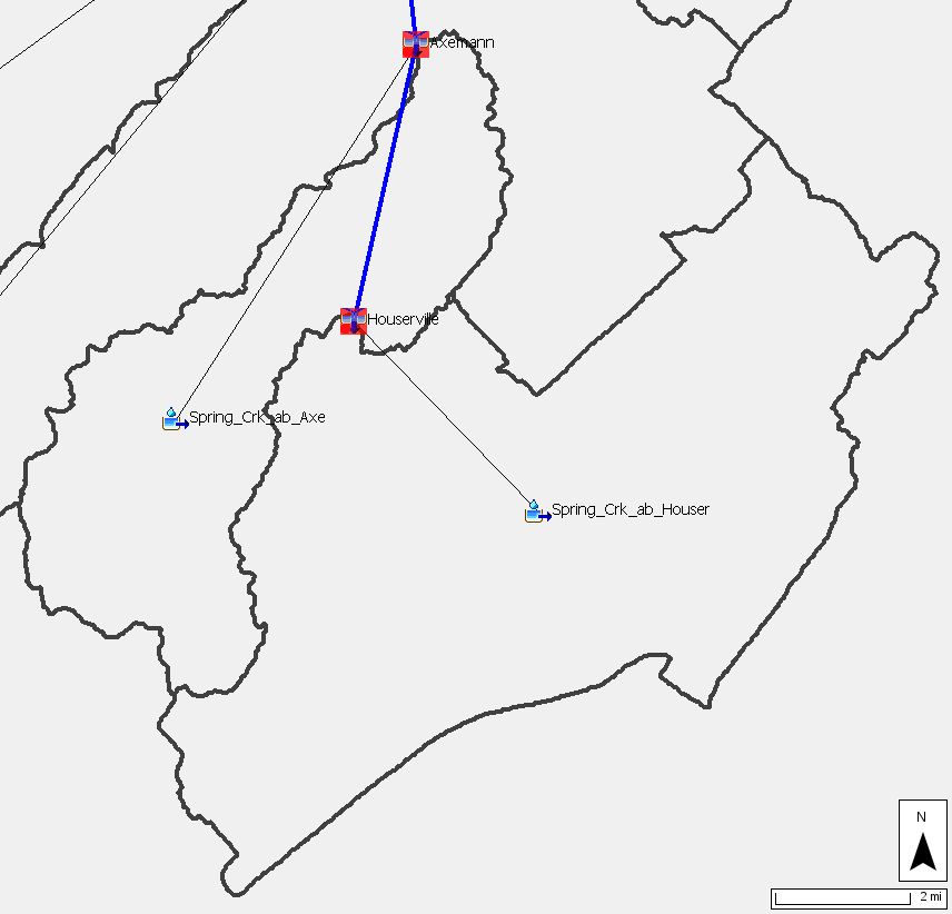
Notice that there are 10 parameters that are already defined. Five of them are related to the "Spring_Crk_ab_Houser" subbasin element and the other five are related to the "Spring_Crk_ab_Axe" subbasin element. This optimization trial is setup to find the parameter sets that best match the observed data at both Houserville and Axeman (located further downstream). Since the Sequential Search option is de-selected, only one optimization routine will be executed with the objective function results at Houserville and Axemann combined and assessed via addition for each iteration.
Navigate to the Search tab. Increase the Max Iterations to 200 and change the Tolerance to 0.1.
Save your project. Compute the "Multi-Location Optimization" simulation. The optimization trial should converge on a solution after roughly 150 iterations.
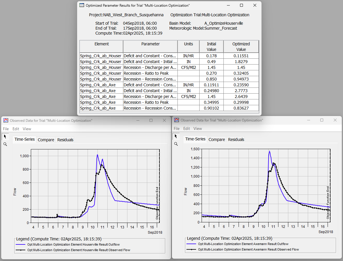
Navigate to the Results tab and expand the "Multi-Location Optimization" simulation node. Notice that there are two folders, one for each specified objective function location. View the Optimized Parameters table and view both of the Observed Data plots contained in the two folders. In this example, the optimization routine did a decent job at converging on a combined parameter set that closely matched the observed data at both locations.

Sequential Searches

Let's explore the Sequential Searches option now. Navigate to the Compute tab and select the "AB_OptimizeHouserAxe" optimization trial.
Navigate to the Objective tab and verify that the Sequential Searches option is selected for Objective Search Type.
Compute the "AB_OptimizeHouserAxe" simulation. Notice in the figure below that the progress bar indicates that two search sequences will take place.

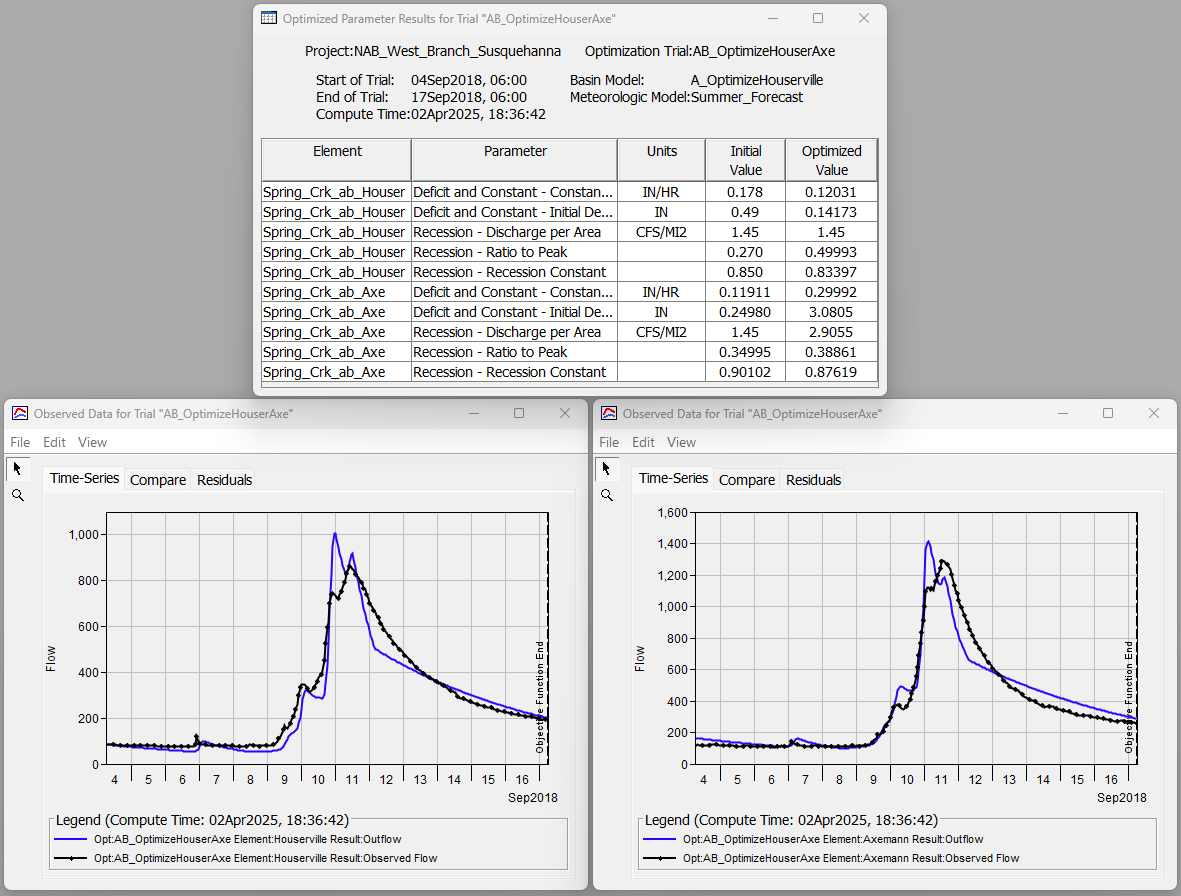
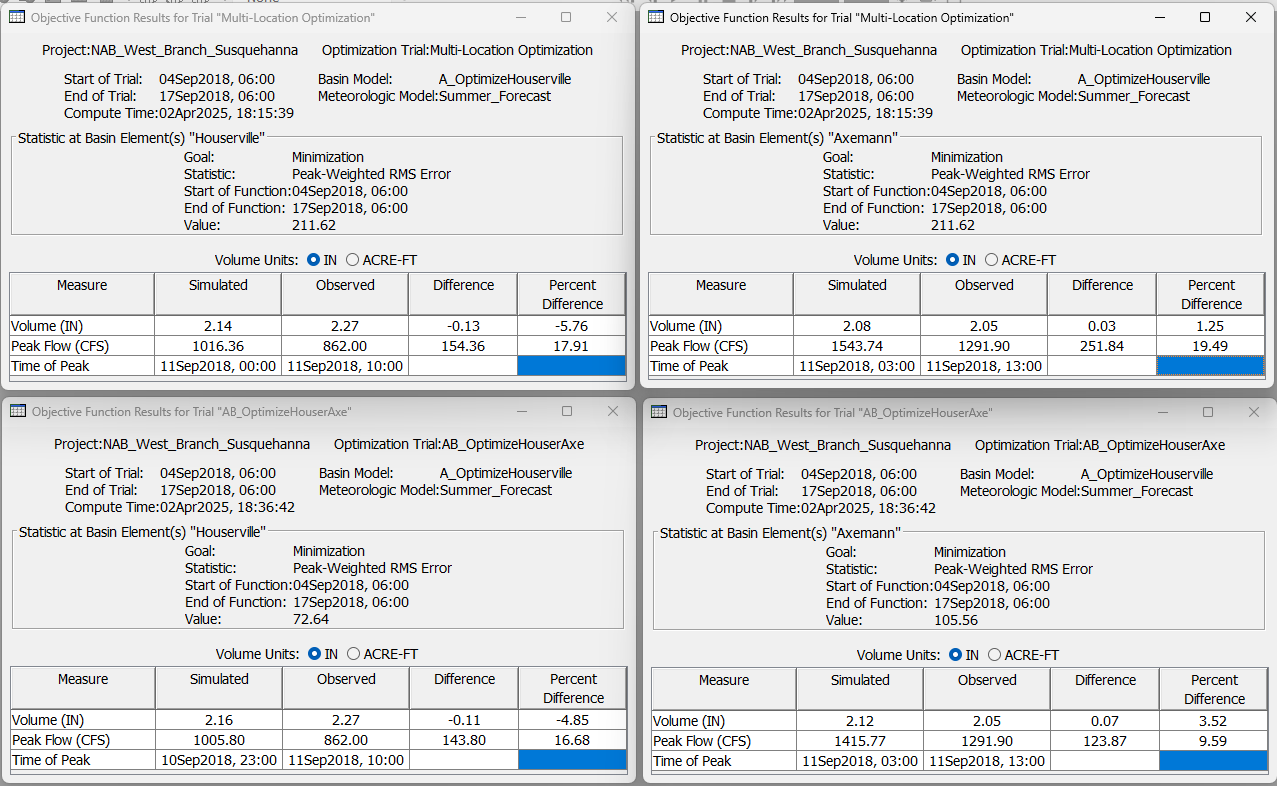
The first search sequence for the Houserville objective should converge on a solution after roughly 130 iterations. The optimized parameter values for "Subbasin_Crk_abv_Houser" are then locked into place and used for the second search sequence at the Axemann objective location further downstream. The second search sequence should converge after roughly 80 iterations.
Navigate to the Results tab and expand the "AB_OptimizeHouserAxe" simulation node. Notice that there are two folders, one for each specified objective function location. View the Optimized Parameters table and view both of the Observed Data plots contained in the two folders. Overall, this optimization trial with the sequential search method performed slightly better than the previously computed "Multi-Location Optimization" trial with the sequential search de-selected. You can use the Objective Function Summary table metrics as well as the calibration metrics on the individual element Summary Table tables to compare and contrast the performance of the two optimization simulations.

Optimization Parameter Types - Subbasin Zone

Let's explore the new "Subbasin Zone" Optimization Parameter type.
Create a copy of the "A_OptimizeHouserville" optimization trial by navigating to the Compute tab, right-clicking the A_OptimizeHouserville node, and selecting Create copy. Name the copy "A_OptimizeHouserville_Zone".
Select and expand the newly created "A_OptimizeHouserville_Zone" node and click on the Parameter 1 node.
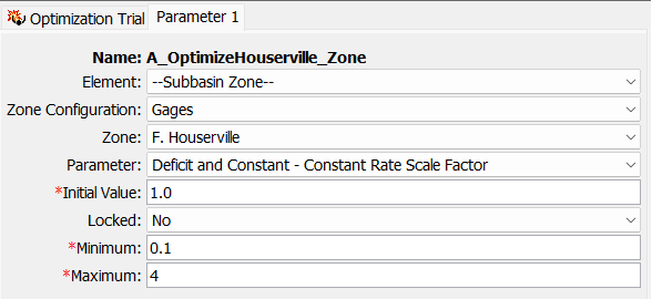
Change the Element to --Subbasin Zone--, the Zone Configuration to Gages, the Zone to F. Houserville, the Parameter to Decit and Constant - Constant Rate Scale Factor, Minimum to 0.1, and Maximum to 4.
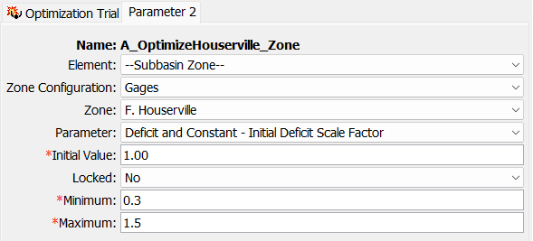
Make similar changes to Parameter 2, but for Parameter select Decit and Constant - Initial Deficit Scale Factor. Enter a Minimum of 0.3 and a Maximum of 1.5
Delete Parameter 3, Parameter 4, and Parameter 5.
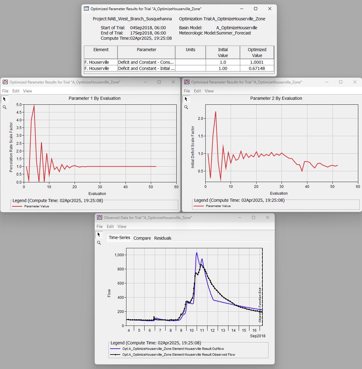
"Subbasin Zone" Optimization Parameters tend to lead to quicker convergence than element-based Optimization Parameters. Decrease the tolerance to 0.0001.
Compute the "A_OptimizeHouserville_Zone" simulation and view the results. In this case, there is only one subbasin element in the F. Houserville Zone ("Spring_Crk_ab_Houser"). So the optimized scale factors are based only on that element. Otherwise, optimized scale factor values that work best considering all elements in the zone would have been determined. In this example, multiplying the constant rate value as defined in the basin model (0.11911 in/hr) by a factor of 1.0001 and the initial deficit value (0.24980 in) by a factor of 0.67148 led to the best results.