Calibration Summary Statistics

HEC-HMS calculates and displays four summary statistics to quantify model performance compared to observations. Statistics include Nash-Sutcliffe Efficiency (NSE), Ratio of the Root Mean Square Error to the Standard Deviation Ratio (RSR) and Percent Bias (PBIAS) (Moriasi, et al., 2007), as well as Coefficient of Determination (R²) (Legates and McCabe, 1999). These statistics are summarized in the Table below. 

Criterion	Equation	Notes
Nash-Sutcliffe Efficiency (NSE)	1) $$//<![CDATA[ \begin{array}{l}\displaystyle NSE=1-\left[\frac{\sum_{i=1}^{n}(Y_i^{obs} - Y_i^{sim})^2} {\sum_{i=1}^{n}(Y_i^{obs} - \bar Y_{obs})^2} \right]\end{array} //]]>$$	NSE evaluates the relative difference between the magnitude of residual data variance ("noise") and the measured data variance (“information”) It is a measure of how well the plot of observed versus simulated data fits the 1:1 line.  Ranges between -$//<![CDATA[ \begin{array}{l}\infty\end{array} //]]>$ and 1. NSE of 1 indicates one-to-one match between the observed and simulated values Negative NSE indicates that the mean of observed values provides a better estimate of the observed data than the model. Widely used in hydrology and is considered a good statistic to represent the overall shape of the hydrograph.
Ratio of the Root Mean Square Error to the Standard Deviation Ratio (RSR)	2) $$//<![CDATA[ \begin{array}{l}\displaystyle RSR=\frac{RMSE}{\sigma_o}=\frac{\left[\sqrt{\sum_{i=1}^{n}(Y_i^{obs}-Y_i^{sim})^2}\right]}{\left[\sqrt{\sum_{i=1}^{n}(Y_i^{obs}-\bar Y_{obs})^2}\right]}\end{array} //]]>$$	Standardizes the root mean square error (RMSE) using the observation standard deviation The optimal value of RSR is 0.0 which presents zero RMSE for perfect model simulation Lower RSR values present better model performance
Percent Bias (PBIAS)	3) $$//<![CDATA[ \begin{array}{l}\displaystyle PBIAS=\left [\frac{\sum_i^n(Y_i^{sim}-Y_i^{obs})*(100)} {\sum_i^n(Y_i^{obs})}\right]\end{array} //]]>$$	Provides a measure of the simulated values are on average larger or smaller than the corresponding observed values. Varies from 0% to infinity, with 0 being the optimal.  Negative PBIAS means the model under-estimates observed data Positive PBIAS means the model over-estimates observed data NOTE: PBIAS sign convention in HEC-HMS is opposite from the sign convention in Moriasi, 2007
Coefficient of Determination (R2)	4) $$//<![CDATA[ \begin{array}{l}\displaystyle R^2=\left[\frac{\sum_i^n(Y_i^{obs}-\bar Y_{obs})(Y_i^{sim}-\bar Y_{sim})}{\sqrt{\sum_i^n(Y_i^{obs}-\bar Y_{obs})^2}*\sqrt{\sum_i^n(Y_i^{sim}-\bar Y_{sim})^2}}\right]^2\end{array} //]]>$$	R2 describes degree of collinearity between simulated and observed data. Represents the proportion of the variance in measured data explained by the model.  Varies between 0 and 1, with 1 being an optimal value. Is oversensitive to outliers and insensitive to additive and proportional differences between model predictions and measured data
Modified Kling Gupta Efficiency (MKGE)	5) $$//<![CDATA[ \begin{array}{l}\displaystyle MKGE = 1 - \sqrt{(r - 1)^2 + (\beta - 1)^2 + (\gamma - 1)^2}\end{array} //]]>$$ 6) $$//<![CDATA[ \begin{array}{l}\displaystyle \beta = \frac{\bar Y_{sim}}{\bar Y_{obs}}\end{array} //]]>$$ 7) $$//<![CDATA[ \begin{array}{l}\displaystyle \gamma= \frac{CV_s}{CV_o} = \frac{\sigma_s/\bar Y_{sim}}{\sigma_o/\bar Y_{obs}}\end{array} //]]>$$	Multi-objective alternative to mean squared error and Nash-Sutcliffe Efficiency (NSE) Can be decomposed into three terms: (1) correlation $//<![CDATA[ \begin{array}{l}r\end{array} //]]>$, (2) bias ratio $//<![CDATA[ \begin{array}{l}\beta\end{array} //]]>$, and (3) variability ratio $//<![CDATA[ \begin{array}{l}\gamma\end{array} //]]>$ The value of MKGE gives the lower limit of the three components ($//<![CDATA[ \begin{array}{l}r\end{array} //]]>$, $//<![CDATA[ \begin{array}{l}\beta\end{array} //]]>$, $//<![CDATA[ \begin{array}{l}\gamma\end{array} //]]>$) The original version of the KGE-statistic uses a variability ratio of γ of σs/σo instead of CVs/CVo. The ratio of coefficient of variations, rather than standard deviations, ensures that the bias and variability ratios are not cross-correlated.

Variables : 

• $//<![CDATA[ \begin{array}{l}Y_i^{obs}\end{array} //]]>$ = i^th observation 
• $//<![CDATA[ \begin{array}{l}Y_i^{sim}\end{array} //]]>$ =  i^th simulated value
• $//<![CDATA[ \begin{array}{l}\bar Y_{obs}\end{array} //]]>$ = the mean of observed data
• $//<![CDATA[ \begin{array}{l}\bar Y_{sim}\end{array} //]]>$ = the mean of simulated data
•  n = total number of observations
• $//<![CDATA[ \begin{array}{l}r\end{array} //]]>$ = correlation coefficient between simulated and observed runoff (dimensionless)
• $//<![CDATA[ \begin{array}{l}\beta\end{array} //]]>$ = bias ratio (dimensionless)
• $//<![CDATA[ \begin{array}{l}\gamma\end{array} //]]>$ = variability ratio (dimensionless)
• $//<![CDATA[ \begin{array}{l}CV\end{array} //]]>$ = coefficient of variation (dimensionless)
• $//<![CDATA[ \begin{array}{l}\sigma\end{array} //]]>$ = standard deviation
• The indices $//<![CDATA[ \begin{array}{l}s\end{array} //]]>$ and $//<![CDATA[ \begin{array}{l}o\end{array} //]]>$ represent simulated and observed runoff values, respectively.

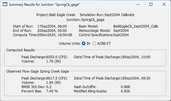
HEC-HMS also reports observed and computed maximum flow, time of peak and total volume. These measures are also useful in the calibration process.

As a reminder, the following basic statistical measures are useful for this discussion:

• Residual variance  = sum of squared differences between the observed and simulated values = $//<![CDATA[ \begin{array}{l}\sum_{i=1}^{n}(Y_i^{obs} - Y_i^{sim})^2\end{array} //]]>$
• Measured data variance = sum of squared differences between the individual observed values and the mean of the observed value = $//<![CDATA[ \begin{array}{l}\sum_{i=1}^{n}(Y_i^{obs} - Y_{obs}^{mean})^2\end{array} //]]>$
• Standard deviation ($//<![CDATA[ \begin{array}{l}\sigma\end{array} //]]>$) is the square root of variance

Performance ranges

Suggested model performance ranges of the four summary statistics for evaluating streamflow, adapted from Moriasi et all, 2007 and 2015, are summarized in the Table below. Note that these are derived for continuous flow data at daily and monthly time steps at watershed scale.

Performance ranges for MKGE are not provided in HEC-HMS. Using the mean flow as a predictor results in a NSE = 0 and a MKGE = 1 - $//<![CDATA[ \begin{array}{l}\sqrt2\end{array} //]]>$ = -0.41. MKGE values greater than -0.41 indicate that the model's performance is better than the mean flow. NSE and MKGE values cannot be directly compared because the relationship depends in part on the coefficient of variation of the observed time series (Knoben et al., 2019). Modelers should analyze the MKGE components (correlation coefficient, bias ratio, and variability ratio) to better understand the model error. 

"What is an acceptable statistical metric?" is an extremely common modeling question and one that elicits considerable debate within the water resources community.  The values presented above and their qualitative interpretations should NOT be blindly used without first considering numerous factors.  These considerations include, but are not limited to, the following: 

• What is the variable(s) of interest (e.g., flow, reservoir pool elevation, snow water equivalent, sediment concentration, etc.)?
• How often are observations taken (e.g., 15 minutes, 1 day, 2 weeks, etc.)?
• What computational time step was used to compute the model results?
• How much uncertainty is present within the observed data and boundary conditions?
• How will model results be used (e.g., $billion infrastructure investment, flood forecasting, evaluation of parameter sensitivity, etc.)?
• What are the time and funding constraints (i.e., can 6 months be invested to calibrate/validate model processes and parameters or must these results be useable within 15 minutes)?

Each modeling application should document which statistical metrics were used to evaluate model performance, their quantitative/qualitative interpretations, and why this was considered appropriate.