Download PDF
Download page Goodness-of-Fit Indices.
Goodness-of-Fit Indices
To compare a computed hydrograph to an observed hydrograph, the program computes an index of the goodness-of-fit. Algorithms included in the program search for the model parameters that yield the best value of an index, also known as objective function. Only one of four objective functions included in the program can be used, depending upon the needs of the analysis. The goal of all four calibration schemes is to find reasonable parameters that yield the minimum value of the objective function. The objective function choices (shown in Table 25) are:
- Sum of absolute errors. This objective function compares each ordinate of the computed hydrograph with the observed, weighting each equally. The index of comparison, in this case, is the difference in the ordinates. However, as differences may be positive or negative, a simple sum would allow positive and negative differences to offset each other. In hydrologic modeling, both positive and negative differences are undesirable, as overestimates and underestimates as equally undesirable. To reflect this, the function sums the absolute differences. Thus, this function implicitly is a measure of fit of the magnitudes of the peaks, volumes, and times of peak of the two hydrographs. If the value of this function equals zero, the fit is perfect: all computed hydrograph ordinates equal exactly the observed values. Of course, this is seldom the case.
- Sum of squared residuals. This is a commonly-used objective function for model calibration. It too compares all ordinates, but uses the squared differences as the measure of fit. Thus a difference of 10 m3/sec "scores" 100 times worse than a difference of 1 m3/sec. Squaring the differences also treats overestimates and underestimates as undesirable. This function too is implicitly a measure of the comparison of the magnitudes of the peaks, volumes, and times of peak of the two hydrographs.
Table 27.Objective functions for calibration.
Criterion | Equation | ||
Sum of absolute errors (Stephenson, 1979) |
| ||
Sum of squared residuals (Diskin and Simon, 1977) |
| ||
Percent error in peak |
| ||
Peak-weighted root mean square error objective function (USACE, 1998) |
|
Note: Z = objective function; NQ = number of computed hydrograph ordinates; q_o(t) = observed flows; q_s(t) = calculated flows, computed with a selected set of model parameters; q_o(peak) = observed peak; q_o(mean) = mean of observed flows; and q_s(peak) = calculated peak
- Percent error in peak. This measures only the goodness-of-fit of the computed-hydrograph peak to the observed peak. It quantifies the fit as the absolute value of the difference, expressed as a percentage, thus treating overestimates and underestimates as equally undesirable. It does not reflect errors in volume or peak timing. This objective function is a logical choice if the information needed for designing or planning is limited to peak flow or peak stages. This might be the case for a floodplain management study that seeks to limit development in areas subject to inundation, with flow and stage uniquely related.
- Peak-weighted root mean square error. This function is identical to the calibration objective function included in computer program HEC-1 (USACE, 1998). It compares all ordinates, squaring differences, and it weights the squared differences. The weight assigned to each ordinate is proportional to the magnitude of the ordinate. Ordinates greater than the mean of the observed hydrograph are assigned a weight greater than 1.00, and those smaller, a weight less than 1.00. The peak observed ordinate is assigned the maximum weight. The sum of the weighted, squared differences is divided by the number of computed hydrograph ordinates; thus, yielding the mean squared error. Taking the square root yields the root mean squared error. This function is an implicit measure of comparison of the magnitudes of the peaks, volumes, and times of peak of the two hydrographs.
In addition to the numerical measures of fit, the program also provides graphical comparisons that permit visualization of the fit of the model to the observations of the hydrologic system. A comparison of computed hydrographs can be displayed, much like that shown in Figure 46. In addition, the program displays a scatter plot, as shown in Figure 47. This is a plot of the calculated value for each time step against the observed flow for the same step. Inspection of this plot can assist in identifying model bias as a consequence of the parameters selected. The straight line on the plot represents equality of calculated and observed flows: If plotted points fall on the line, this indicates that the model with specified parameters has predicted exactly the observed ordinate. Points plotted above the line represents ordinates that are over-predicted by the model. Points below represent under-predictions. If all of the plotted values fall above the equality line, the model is biased; it always over-predicts. Similarly, if all points fall below the line, the model has consistently under-predicted. If points fall in equal numbers above and below the line, this indicates that the calibrated model is no more likely to over-predict than to under-predict.
The spread of points about the equality line also provides an indication of the fit of the model. If the spread is great, the model does not match well with the observations – random errors in the prediction are large relative to the magnitude of the flows. If the spread is small, the model and parameters fit better.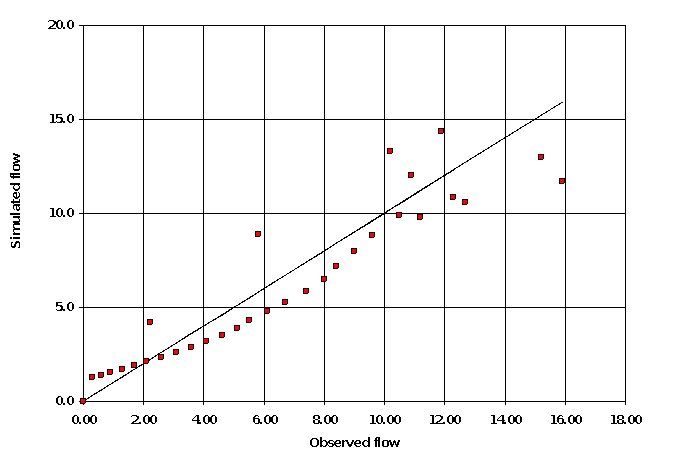
Figure 52.Scatter plot of optimization results.
The program also computes and plots a time series of residuals—differences between computed and observed flows. Figure 48 is an example of this. This plot indicates how prediction errors are distributed throughout the duration of the simulation. Inspection of the plot may help focus attention on parameters that require additional effort for estimation. For example, if the greatest residuals are grouped at the start of a runoff event, the initial loss parameter may have been poorly chosen.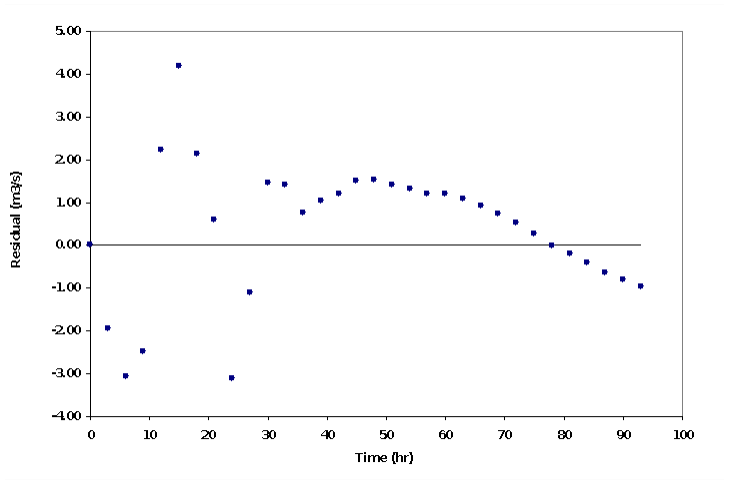
Figure 53.Residual plot of optimization results.