Search Methods

As noted earlier, the goal of calibration is to identify reasonable parameters that yield the best fit of computed to observed hydrograph, as measured by one of the objective functions. This corresponds mathematically to searching for the parameters that minimize the value of the objective function.
As shown in Figure 45, the search is a trial-and-error search. Trial parameters are selected, the models are exercised, and the error is computed. If the error is unacceptable, the program changes the trial parameters and reiterates. Decisions about the changes rely on the univariate gradient search algorithm or the Nelder and Mead simplex search algorithm.

Univariate-Gradient Algorithm

The univariate-gradient search algorithm makes successive corrections to the parameter estimate. That is, if $\begin{array}{l}x^k\end{array}$ represents the parameter estimate with objective function $\begin{array}{l}f(x^k)\end{array}$ at iteration k, the search defines a new estimate $\begin{array}{l}x^{k+1}\end{array}$ at iteration k+1 as:

$\begin{array}{l}\displaystyle x^{k+1}=x^k+\Delta x^k\end{array}$

in which $\begin{array}{l}\Delta x^k\end{array}$ = the correction to the parameter. The goal of the search is to select $\begin{array}{l}\Delta x^k\end{array}$ so the estimates move toward the parameter that yields the minimum value of the objective function. One correction does not, in general, reach the minimum value, so this equation is applied recursively.
The gradient method, as used in the program, is based upon Newton's method. Newton's method uses the following strategy to define $\begin{array}{l}\Delta x^k\end{array}$ :

The objective function is approximated with the following Taylor series:

$\begin{array}{l}\displaystyle f\left(x^{k+1}\right)=f\left(x^{k}\right)+\left(x^{k+1}-x^{k}\right) \frac{d f\left(x^{k}\right)}{d x}+\frac{\left(x^{k+1}-x^{k}\right)^{2}}{2} \frac{d^{2} f\left(x^{k}\right)}{d x^{2}}\end{array}$

in which $\begin{array}{l}f(x^{k+1})\end{array}$ = the objective function at iteration k; and $\begin{array}{l}\frac{df(x^k)}{dx}\end{array}$ and $\begin{array}{l}\frac{d^2f(x^k)}{ds^2}\end{array}$ = the first and second derivatives of the objective function, respectively.

Ideally, $\begin{array}{l}x^{k+1}\end{array}$ should be selected so $\begin{array}{l}f(x^{k+1})\end{array}$ is a minimum. That will be true if the derivative of $\begin{array}{l}f(x^{k+1})\end{array}$ is zero. To find this, the derivative of Equation 107 is found and set to zero, ignoring the higher order terms. That yields

$\begin{array}{l}\displaystyle 0=\frac{d f\left(x^{k}\right)}{d x}+\left(x^{k+1}-x^{k}\right) \frac{d^{2} f\left(x^{k}\right)}{d x^{2}}\end{array}$

This equation is rearranged and combined with Equation 106, yielding

$\begin{array}{l}\displaystyle \Delta x^{k}=-\frac{\frac{d f\left(x^{k}\right)}{d x}}{\frac{d^{2} f\left(x^{k}\right)}{d x^{2}}}\end{array}$

The program uses a numerical approximation of the derivatives $\begin{array}{l}\frac{df(x^k)}{dx}\end{array}$ and $\begin{array}{l}\frac{d^2f(x^k)}{dx^2}\end{array}$ at each iteration k. These are computed as follows:

Two alternative parameters in the neighborhood of $\begin{array}{l}x^k\end{array}$ are defined as $\begin{array}{l}x^{k_1}\end{array}$ = $\begin{array}{l}0.99x^k\end{array}$ and $\begin{array}{l}x^{k_2}\end{array}$ = $\begin{array}{l}0.98x^{k_2}\end{array}$ , and the objective function value is computed for each.
Differences are computed, yielding $\begin{array}{l}\Delta_1\end{array}$ = $\begin{array}{l}f(x^{k_1})\end{array}$ – $\begin{array}{l}f(x^k)\end{array}$ and $\begin{array}{l}\Delta_2\end{array}$ = $\begin{array}{l}f(x^{k_2})\end{array}$ – $\begin{array}{l}f(x^{k_1})\end{array}$
The derivative $\begin{array}{l}\frac{df(x^k)}{dx}\end{array}$ is approximated as $\begin{array}{l}\Delta_1\end{array}$ , and $\begin{array}{l}\frac{d^2f(x^k)}{dx^2}\end{array}$ is approximated as $\begin{array}{l}\Delta_2-\Delta_1\end{array}$ . Strictly speaking, when these approximations are substituted in Equation 109, this yields the correction $\begin{array}{l}\Delta x^k\end{array}$ in Newton's method.

As implemented in the program, the correction is modified slightly to incorporate HEC staff experience with calibrating the models included. Specifically, the correction is computed as:
$\begin{array}{l}\Delta x^k=0.01Cx^k\end{array}$
in which C is as shown in Table 26.
In addition to this modification, the program tests each value $\begin{array}{l}x^{k+1}\end{array}$ to determine if, in fact, $\begin{array}{l}f(x^{k+1})\end{array}$ < $\begin{array}{l}f(x^k)\end{array}$ . If not, a new trial value, $\begin{array}{l}x^{k+2}\end{array}$ is defined as

$\begin{array}{l}\displaystyle x^{k+2}=0.7x^k+0.3x^{k+1}\end{array}$

If $\begin{array}{l}f(x^{k+2})\end{array}$ > $\begin{array}{l}f(x^k)\end{array}$ , the search ends, as no improvement is indicated.

Table 28.Coefficients for correction in the univariant gradient search.

$\begin{array}{l}\Delta_2-\Delta_1\end{array}$	$\begin{array}{l}\Delta_1\end{array}$	C
> 0	—	$\begin{array}{l}\frac{\Delta_1}{\Delta_2}-0.5\end{array}$
< 0	> 0	50
	$\begin{array}{l}\leq\end{array}$ 0	-33

If more than a single parameter is to be found via calibration, this procedure is applied successively to each parameter, holding all others constant. For example, if Snyder's Cp and tp are sought, Cp, is adjusted while holding tp at the initial estimate. Then, the algorithm will adjust tp, holding Cp at its new, adjusted value. This successive adjustment is repeated four times. Then, the algorithm evaluates the last adjustment for all parameters to identify the parameter for which the adjustment yielded the greatest reduction in the objective function. That parameter is adjusted, using the procedure defined here. This process continues until additional adjustments will not decrease the objective function by at least 1%.

Nelder and Mead Algorithm

The Nelder and Mead algorithm searches for the optimal parameter value without using derivatives of the objective function to guide the search. Instead this algorithm relies on a simpler direct search. In this search, parameter estimates are selected with a strategy that uses knowledge gained in prior iterations to identify good estimates, to reject bad estimates, and to generate better estimates from the pattern established by the good.
The Nelder and Mead search uses a simplex—a set of alternative parameter values. For a model with n parameters, the simplex has n+1 different sets of parameters. For example, if the model has two parameters, a set of three estimates of each of the two parameters is included in the simplex. Geometrically, the n model parameters can be visualized as dimensions in space, the simplex as a polyhedron in the n-dimensional space, and each set of parameters as one of the n+1 vertices of the polyhedron. In the case of the two-parameter model, then, the simplex is a triangle in two-dimensional space, as illustrated in Figure 49.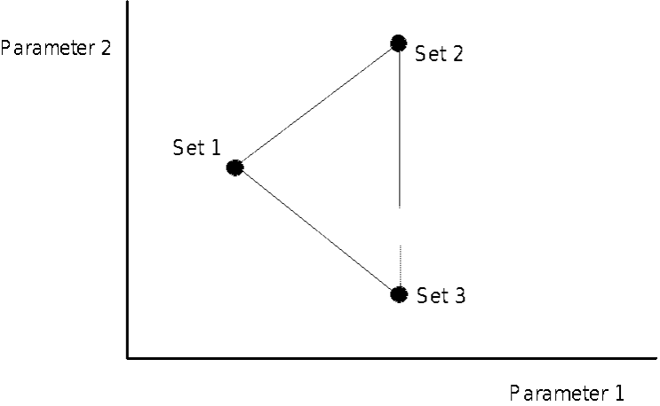

Figure 54.Initial simplex for a 2-parameter model.
The Nelder and Mead algorithm evolves the simplex to find a vertex at which the value of the objective function is a minimum. To do so, it uses the following operations:

Comparison. The first step in the evolution is to find the vertex of the simplex that yields the worst (greatest) value of the objective function and the vertex that yields the best (least) value of the objective function. In Figure 50, these are labeled W and B, respectively.
Reflection. The next step is to find the centroid of all vertices, excluding vertex W; this centroid is labeled C in Figure 50. The algorithm then defines a line from W, through the centroid, and reflects a distance WC along the line to define a new vertex R, as illustrated Figure 50.

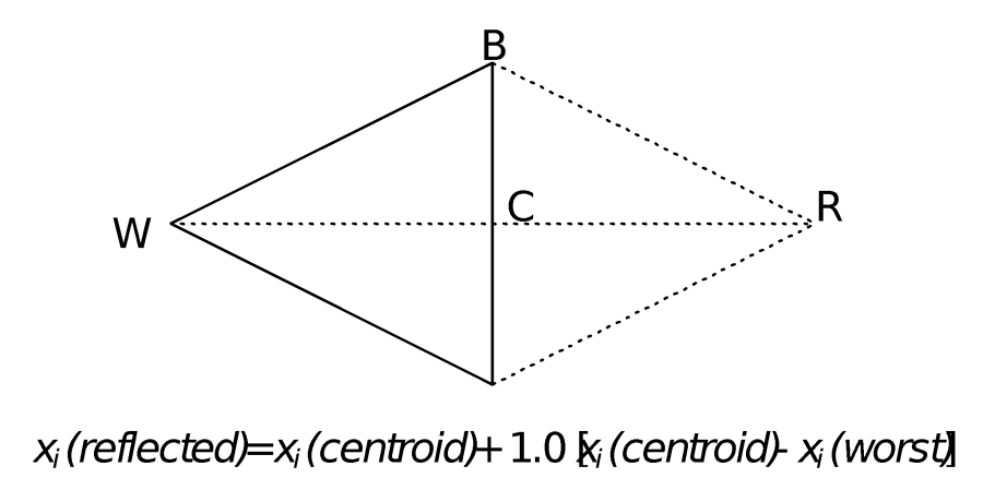
Figure 55.Reflection of a simplex.

Expansion. If the parameter set represented by vertex R is better than, or as good as, the best vertex, the algorithm further expands the simplex in the same direction, as illustrated in Figure 51. This defines an expanded vertex, labeled E in the figure. If the expanded vertex is better than the best, the worst vertex of the simplex is replaced with the expanded vertex. If the expanded vertex is not better than the best, the worst vertex is replaced with the reflected vertex.

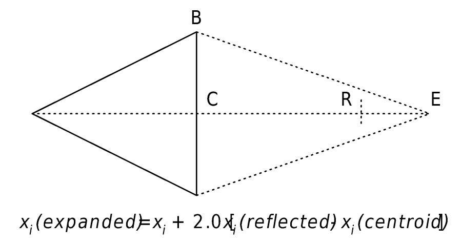
Figure 56.Expansion of a simplex.

Contraction. If the reflected vertex is worse than the best vertex, but better than some other vertex (excluding the worst), the simplex is contracted by replacing the worst vertex with the reflected vertex. If the reflected vertex is not better than any other, excluding the worst, the simplex is contracted. This is illustrated in Figure 52. To do so, the worst vertex is shifted along the line toward the centroid. If the objective function for this contracted vertex is better, the worst vertex is replaced with this vertex.

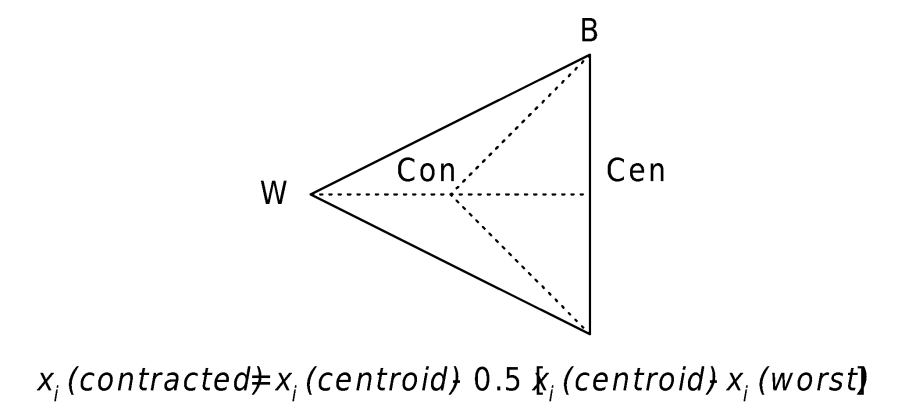
Figure 57.Contraction of a simplex.

Reduction. If the contracted vertex is not an improvement, the simplex is reduced by moving all vertices toward the best vertex. This yields new vertices R₁ and R₂, as shown in Figure 53.

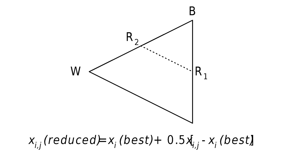
Figure 58.Reduction of a simplex.

The Nelder and Mead search terminates when either of the following criterion is satisfied:

$\begin{array}{l}\displaystyle \sqrt{\sum_{j=1, j \mid \text { rost }}^{n} \frac{\left(z_{j}-z_{c}\right)^{2}}{n-1}< \text { tolerance }}\end{array}$

in which n = number of parameters; j = index of a vertex, c = index of centroid vertex; and $\begin{array}{l}z_j\end{array}$ and $\begin{array}{l}z_c\end{array}$ = objective function values for vertices j and c, respectively.

The number of iterations reaches 50 times the number of parameters.

The parameters represented by the best vertex when the search terminates are reported as the optimal parameter values.