Download PDF
Download page Ensemble Modeling.
Ensemble Modeling
Basic Concepts
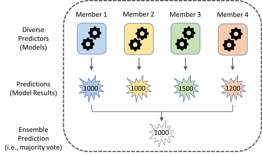
In general, an ensemble model is a collection of multiple, diverse models that are created to predict a similar outcome. An ensemble model can be composed of 2 to many base models which are often referred to as ensemble members. There are two key components involved in ensemble modeling: 1) the selection of the ensemble members and 2) the aggregation of the ensemble member predictions (individual model results or traces) into an ensemble model prediction. In the below figure, an ensemble model comprised of four ensemble members is depicted. In this example, the ensemble member predictions are aggregated into an ensemble prediction by a simple, majority vote.

One of the main reasons to use ensemble modeling is to reduce uncertainty in the modelled predictions. As a general rule of thumb, ensemble models tend to outperform single-algorithm models. The ability to see multiple ensemble member traces each of which represent a viable, possible outcome is a powerful modeling feature. It allows modelers and decision-makers the ability to analyze and act on a range of possible outcomes as opposed to only seeing one possible outcome with a potentially large amount of uncertainty.
When selecting ensemble members, each member should be performant. Each should be designed and equipped to accurately model the intended outcome/goal of the overall ensemble model. For example, if the study goal is to model the 1% AEP (annual exceedance probability) rainfall-runoff event at a given location, individual models that were only designed/calibrated to predict relatively common, low-flow events should not be included as ensemble members. Furthermore, each ensemble member should be independent. It is most desirable to include ensemble members that are constructed in fundamentally different ways and/or that make different assumptions; independent members lead to less correlated prediction errors.
There are multiple ways to aggregate individual ensemble member results into an overall ensemble model prediction. One of the simplest and most commonly used methods is to average the ensemble member results treating each result equally. Weighted average techniques can also be applied by assigning weights to favor the strongest ensemble members and to disfavor the weakest. There are many advanced statistical techniques that can be used for bias correction with observed data, each having the same end goal of leveraging the ensemble members that perform best historically.
Ensemble Modeling in HEC-HMS
In HEC-HMS, the power of ensemble modeling can be leveraged via the Ensemble Analysis compute type. Currently, ensemble members within an ensemble analysis may consist of either Simulation Runs or Forecast Alternatives. Since a simulation run or forecast alternative each have a basin model and a meteorologic model associated with them, there are a wide variety of ways that an ensemble analysis can be applied.
One general approach is to build an analysis with members that use the same basin model but different meteorologic models. For example, each member could be assigned a unique meteorologic model that represents a different forecasted precipitation dataset. By building and computing an ensemble analysis in this fashion, it would highlight the uncertainty present within the different forecast models and demonstrate how flow results at a downstream point of interest might vary.
A second general approach is to build an ensemble analysis with members that use the same meteorologic model but different basin models. For example, the same hypothetical storm event could be applied to each ensemble member, but each member could reference a different basin model that represents a specific antecedent condition such as wet, dry, or normal. By building and computing an ensemble analysis in this fashion, it would highlight how sensitive rainfall-runoff results might be depending on the antecedent state a watershed is in when a storm event occurs.
There are many different ways in which an ensemble analysis can be constructed and applied, each affording the modeler with the benefits of additional insight and reduced uncertainty in the modeling results. Currently in HEC-HMS, ensemble member predictions can be aggregated for the following time-series types:
- Incremental Precipitation
- Cumulative Precipitation
- Outflow
- Cumulative Outflow
- Reservoir Elevation
- Moisture Deficit
- SWE (snow-water equivalent)
- LWASS (liquid-water at soil surface)
- Air Temperature
- Sediment Load (total amounts and individual amounts for clay, silt, sand, gravel, cobble and boulder)
- Sediment Volume (total amounts and individual amounts for clay, silt, sand, gravel, cobble and boulder).
The current ensemble model aggregation options in HEC-HMS include the following:
- Mean
- +/- one standard deviation
- Maximum
- Minimum.
Ensemble Viewer
Additional aggregation options and visualization capabilities are present within the Ensemble Viewer which is accessible in HEC-HMS via the Tools dropdown on the main menu bar.
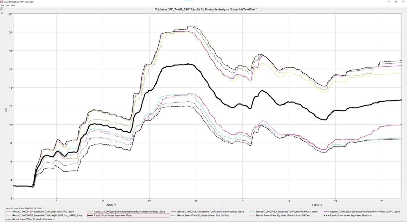
The below figure represents an ensemble analysis results plot of SWE. This plot highlights how SWE could potentially vary based on the precipitation dataset that is applied as a boundary condition. Even though the precipitation datasets model the same event period, they can yield noticeably different results. The individual ensemble member results for SWE are shown in the colored lines whereas the aggregated ensemble model predictions are shown in the black, dotted lines.

There are several tutorials and guides available for the Ensemble Analysis that highlight different applications such as flood forecasting and climate modeling. They can be found here: Ensemble Analysis Simulations in HEC-HMS.