Download PDF
Download page Inverse Distance Gage Weighting.
Inverse Distance Gage Weighting
The inverse distance gage weighting method was originally designed for real-time forecasting applications. It includes procedures for automatically using the closest available gage data, but switching to more remote gages if close gages stop reporting or contain missing data.
Basic Concepts and Equations
As an alternative to separately defining the total mean areal precipitation (MAP) depth and combining this with a pattern temporal distribution to derive the MAP hyetograph, one can select a scheme that computes the MAP hyetograph directly. This so-called inverse-distance-squared weighting method computes P(t), the subbasin precipitation at time t, by dynamically applying a weighting scheme to precipitation measured at watershed precipitation gages at time t.
The scheme relies on the notion of nodes that are positioned within a subbasin such that they provide adequate spatial resolution of precipitation in the subbasin. The program computes the precipitation hyetograph for each node using gages near that node. To select these gages, hypothetical north-south and east-west axes are constructed through each node and the nearest gage is found in each quadrant defined by the axes. This is illustrated in Figure 15. Weights are computed and assigned to the gages in inverse proportion to the square of the distance from the node to the gage. For example, in Figure 15, the weight for the gage C in the northeastern quadrant of the grid is computed as:
| $w_{C}=\frac{\frac{1}{d_{C}^{2}}}{\frac{1}{d_{C}^{2}}+\frac{1}{d_{D}^{2}}+\frac{1}{d_{E}^{2}}+\frac{1}{d_{A}^{2}}}$ |
in which wC = weight assigned to gage C; dC = distance from node to gage C; dD = distance from node to gage D in southeastern quadrant; dE = distance from node to gage E in southwestern quadrant; and dF = distance from node to gage F in northwestern quadrant of grid. Weights for gages D, E and A are computed similarly. The distance between each gage and the node is computed using a curved earth assumption as:
| $d=r a d \cdot \cos ^{-1}(\cos (A) \cdot \cos (B)+\sin (A) \cdot \sin (B) \cdot \cos (C))$ |
where d is the distance between a gage and the node; rad is the radius of the earth at 6370 km; A is one-half pi minus latitude of the gage in radians, B is one-half pi minus the latitude of the node in radians, and C is the longitude of the node in radians minus the longitude of the gage.
With the weights thus computed, the node hyetograph ordinate at time t is computed as:
| $p_{\text {node }}(t)=w_{A} p_{A}(t)+w_{C} p_{C}(t)+w_{D} p_{D}(t)+w_{E} p_{E}(t)$ |
This computation is repeated for all times t. Note that gage B in Figure 15 is not used in this example, as it is not nearest to the node in the northwestern quadrant. However, for any time that the precipitation ordinate is missing for gage A, the data from gage B will be used. In general terms, the nearest gage in the quadrant with data (including a zero value) will be used to compute the MAP.
Figure 15.Illustration of inverse-distance-squared scheme.
As noted in the description of the user-specified gage weights method, regional trends in meteorology and specifically precipitation can lead to problems. The index precipitation can be used to account for these trends. Each node can have an index depth as well as each gage. The index correction can only be used if it is specified for all gages and nodes that will be used for a subbasin. When used, the index precipitation values are included in the calculations as:
| $p_{n o d e}(t)=\frac{I_{n o d e} w_{A}}{I_{A}} p_{A}(t)+\frac{I_{n o d e} w_{C}}{I_{c}} p_{c}(t)+\frac{I_{n o d e} w_{D}}{I_{D}} p_{D}(t)+\frac{I_{n o d e} w_{E}}{I_{E}} p_{E}(t)$ |
Where Inode is the index at the node, IA is the index at gage A, and IC, ID, and IE are the index at each of the remaining gages.
This example has used only one node in the subbasin. However, it is possible to include more than one node. In this case a weight must be specified for each node as the final precipitation hyetograph for the subbasin is computed as:
| $p(t)=\sum_{i} w_{i} p_{i}(t)$ |
Where p(t) is the precipitation at each time t for the subbasin; wi is the weight for node i; pi(t) is the precipitation at each time t for node i as computed by equation 10. Node weights will need to add to 1. Node weights must sum up to 1; in cases where weights surpass this value, the software will automatically normalize the weights to ensure their collective sum equals 1.
Most recording gages that are used with this method report data at a 1-hour or shorter interval. However, there are many gages available that only report once a day, giving the total daily precipitation. These gages can also be used for calculating the precipitation at each node. Each "daily" gage is preprocessed before beginning the calculations for a node. The processed daily gage is used exactly as if it were a recording gage when dynamically computing the precipitation for each node.
The preprocessing for a daily gage utilizes recording gages near the daily gage to compute a pattern hyetograph and then applies the precipitation recorded at the daily gage. The processing is similar to what happens at a node. Hypothetical north-south and east-west axes are constructed through the coordinates of the daily gage. The adjacent recording gages are sorted into each of the four quadrants surrounding the daily gage. The closest gage is selected in each quadrant; this process is performed once and not for each time interval as is done when processing for a node. For each time step, pattern precipitation is computed at the daily gage using equations 7, 8, and 10 with the substitution of the daily gage coordinates for the node coordinates. Subsequently, the pattern precipitation hyetograph is normalized by dividing each value by the total depth in the pattern precipitation. This step yields a pattern hyetograph for the daily gage that has exactly 1 unit of precipitation depth. The next step in preprocessing the daily gage is to determine the total depth recorded at the daily gage. Only time intervals at the daily gage that are completely within the simulation time window are included for computing the total depth. For example, consider a daily gage that is used in a simulation at begins on the first day at 12:00 hours and continues until 12:00 hours on the fifth day. Only the daily gage values recorded on the second through fourth days will be included. This is necessary because it is not possible to know when the depth recorded by the daily gage on the first day happened during the day. It is possible that it occurred during the first 12 hours of the day which are not included in the simulation time window, so they must be excluded. Each value in the normalized pattern hyetograph is multiplied by the calculated total depth at the daily gage to yield the final gage hyetograph used in node calculations.
Parameter Estimation
This method requires at least one node for each subbasin. The parameters then are the latitude and longitude of the node and any gages that will be used. The coordinates of each gage are generally known or can be found by examining a map. The use of the index precipitation is optional.
Selecting Node Locations
A common practice is to specify a single node for each subbasin, located at the centroid of the subbasin. This can be a quick way to initially estimate parameters because it is relatively easy to compute the coordinates of the subbasin centroid using a geographic information system. This is less arbitrary that it first seems. By definition, the centroid is closer to more of the subbasin than any other point. Using this placement assumes that centering in the subbasin is the best representation of the subbasin-average precipitation.
An alternate method of placing the node would be to examine the precipitation trends over the subbasin. Compute the average annual subbasin precipitation by consulting regional maps. One source for such maps is the PRISM project (Daly, Neilson, and Phillips, 1994) which includes both total annual and monthly estimates of precipitation. Once the average annual precipitation amount for the subbasin is known, a node could be located at a point in the subbasin with the same average annual precipitation depth. Ideally, the selected point would be near the centroid. This placement attempts to match individual storm events that will be simulated consistent with the average trends in the subbasin.
Regardless of the method used to locate the node, placement should consider the surrounding gages. Sometimes the location initially selected for the node will almost always ignore a gage that is relatively close, as shown in Figure 16. Because of the node placement, all four gages fall into only three quadrants. Most of the time only the three closest gages will be used and gage B will never be used unless there is missing data at gage A. By moving the node slightly East, each gage will fall into a separate quadrant and be used.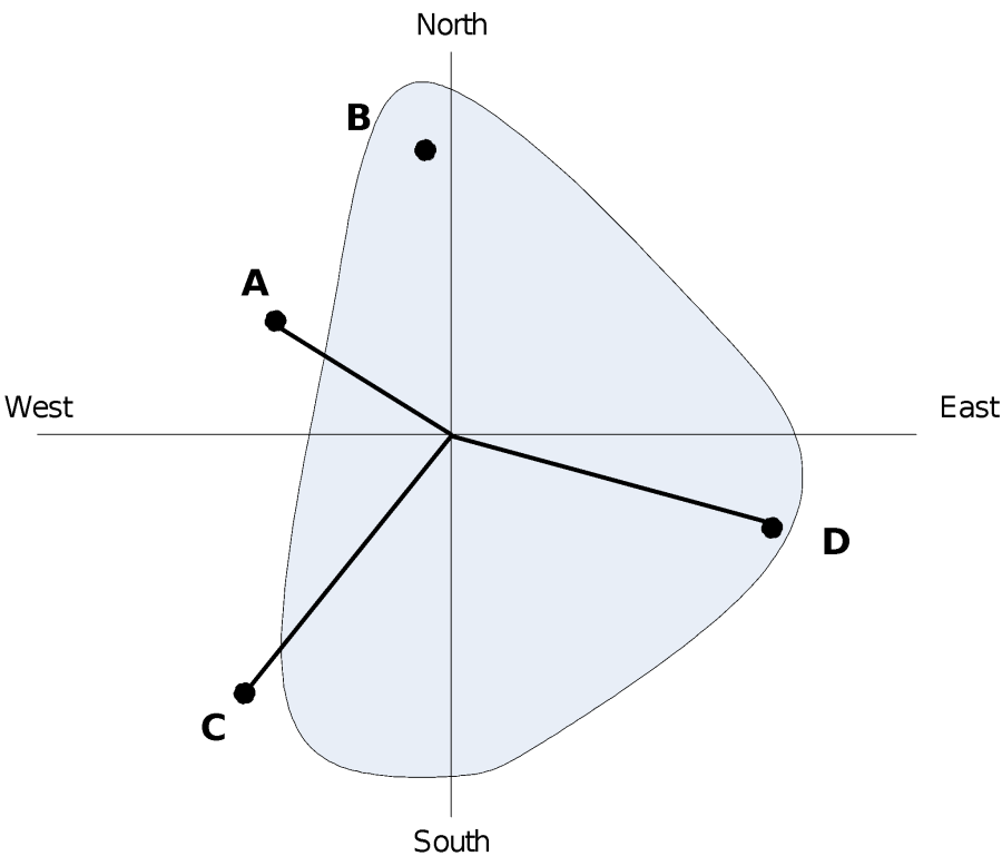
Figure 16.Placing a subbasin node where one gage is excluded. Moving the node to the West would use all four gages.
It is possible to use more than one node in a subbasin. However, if two or more nodes are used, the pattern for the subbasin will be a weighted average of that computed at those nodes. Consequently, if the temporal distribution at those nodes is significantly different, as it might be with a moving storm, the average pattern may obscure information about the precipitation intensity over the subbasin. If circumstances cause precipitation patterns to differ significantly over a subbasin so that multiple nodes may be necessary, it is often better to subdivide the subbasin rather than use multiple nodes.
Daily Gages
Strictly speaking, any gage can be considered a "recording" or "daily" gage. A recording gage will be interpolated in time in order to obtain values at the time step of the simulation. As an example, consider a recording gage with data recorded at 1-hour intervals. If the simulation is computed at a 15-minute time interval, then each value in the gage time-series will be divided into four equal amounts during each hour in order to have a value for each simulation time step. This so-called down scaling can be an acceptable approximation of the precipitation but the approximation becomes worse as the ratio of simulation time interval divided by the gage recording interval becomes smaller. It is a fact that gages cannot capture information about the temporal distribution of precipitation at time scales smaller than the recording interval of the gage.
As a second example, consider a gage that records data at a 1-day time interval that will be used in a simulation with a 1-hour time step. If the gage were treated as a typical recording gage, each daily value would be divided into 24 equal values for the simulation time step during each day. In general, this would lead to unacceptable smoothing of the daily data. Designating the gage as "daily" will allow the processing described above to convert the data to a better approximation of what happened at short time scale by using adjacent high-resolution gages.
You should always have at least one gage with a data time interval near the simulation time interval. Any gage with a data time interval more than several times the simulation time interval should be evaluated for treatment as a "daily" gage. For example, if the simulation time interval is 1-hour and some gages report at 6-hour intervals, they should be evaluated for treatment as daily gages. Even though they report at less that 24-hour or daily intervals, their time interval is so much longer than the simulation interval that results may be significantly improved by using the "daily" processing option.