Shortwave radiation is a radiant energy produced by the sun with wavelengths ranging from infrared through visible to ultraviolet. Shortwave radiation is therefore exclusively associated with daylight hours for a particular location on the Earth's surface. The energy arrives at the top of the Earth's atmosphere with a flux (Watts per square meter) that varies very little during the year and between years. Consequently the flux is usually taken as a constant for hydrologic simulation purposes. Some of the incoming radiation is reflected by the top of the atmosphere and some is reflected by clouds. A portion of the incoming radiation is absorbed by the atmosphere and some is absorbed by clouds. The albedo is the fraction of the shortwave radiation arriving at the land surface that is reflected back into the atmosphere. The shortwave radiation that is not reflected or absorbed above the land surface, and is not reflected by the land surface, is available to drive hydrologic processes such as evapotranspiration and snowpack melting.

The shortwave radiation method included in the meteorologic model is only necessary when energy balance methods are used for evapotranspiration or snowmelt. The options available cover a range of detail from simple to complex. Simple specified methods are also available for input of a time-series gage or grid. Each option produces the net shortwave radiation arriving at the land surface where it may be reflected or absorbed. More detail about each method is provided in the following sections.

Bristow Campbell

The Bristow Campbell method (Bristow and Campbell, 1984) uses a conceptual approach to estimating the shortwave radiation at the land surface. During the daylight hours, any clouds present in the atmosphere will block some portion of incoming solar radiation which reduces solar heating and results in a lower temperature. Conversely, lack of clouds permits much more of the solar radiation to pass through the atmosphere which allows greater heating and generally higher air temperatures. In theory, the daily temperature range should be small on cloudy days and large on non-cloudy days. This correlation between temperature range and incoming solar radiation is exploited as a simple way to compute shortwave radiation using only air temperature.

The Bristow Campbell method includes a Component Editor with parameter data for each subbasin in the meteorologic model. The Watershed Explorer provides access to the shortwave component editor using a picture of solar radiation (Figure 1).

An air temperature gage must be selected in the atmospheric variables for each subbasin.

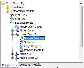
Figure 1. A meteorologic model using the Bristow Campbell shortwave radiation method with a component editor for each individual subbasin.

The Component Editor for each subbasin in the meteorologic model is used to enter parameter data (Figure 2). The transmittance represents the maximum clear sky characteristics over the watershed. The default value of the transmittance is 0.70. The exponent controls the timing of the maximum temperature and may vary from humid to arid environments. The default value of the exponent is 2.4.

The average monthly temperature range must be entered. This value is the difference between the average monthly high temperature and the average monthly low temperature.

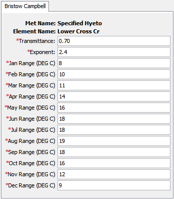
Figure 2. Entering atmosphere and temperature data for a subbasin using the Bristow Campbell shortwave radiation method.

FAO56

The FAO56 method implements the algorithm detailed by Allen, Pereira, Raes, and Smith (1998). The algorithm calculates the solar declination and solar angle for each time interval of the simulation, using the coordinates of the subbasin, Julian day of the year, and time at the middle of the interval. The solar values are used to compute the extra-terrestrial radiation for each subbasin. Total daylight hours are computed based on the Julian day and compared to the number of actual sunshine hours. Shortwave radiation arriving at the ground surface is then computed using the most common relationship accounting for reduction in sunshine hours due to cloud cover.

The Watershed Explorer provides access to the shortwave component editors using a picture of solar radiation (Figure 3). The FAO56 method includes a Component Editor with parameter data for all subbasins in the meteorologic model (Figure 4). A Component Editor is also included for each subbasin (Figure 5).

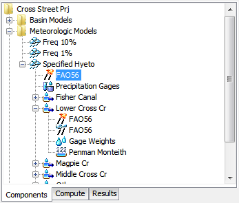
Figure 3. A meteorologic model using the FAO56 shortwave radiation method with a component editor for each individual subbasin.

A Component Editor for all subbasins in the meteorologic model includes the central meridian of the time zone (Figure 4). There is currently no specification for the time zone so the meridian must be specified manually. The central meridian is commonly the longitude at the center of the local time zone. Meridians west of zero longitude should be specified as negative while meridians east of zero longitude should be specified as positive. The meridian may be specified in decimal degrees or degrees, minutes, and seconds depending on the program settings.

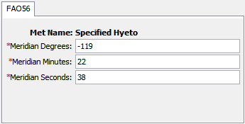
Figure 4. Entering the longitude of the central meridian of the local time zone.

The Component Editor for each subbasin in the meteorologic model is used to enter parameter data necessary to account for differences in cloud cover across the watershed (Figure 5). Cloud cover is considered through a time-series of sunshine hours. Sunshine hours are defined as the number of decimal hours per full hour where the shortwave radiation exceeds 120 watts per square meter (WMO, 2008).

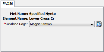
Figure 5. Selecting a time-series gage for the sunshine hours.

Gridded Hargreaves

The gridded Hargreaves method is the same as the regular Hargreaves method (described in a later section) except that the Hargreaves equations are applied to each grid cell using separate boundary conditions instead of area-averaged values over the whole subbasin.

The gridded Hargreaves shortwave method includes a Component Editor with parameter data for all subbasins in the meteorologic model. The Watershed Explorer provides access to the shortwave component editor using a picture of solar radiation (Figure 6).

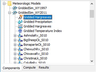
Figure 6. A meteorologic model using the gridded Hargreaves shortwave method with a component editor for all subbasins.

The Component Editor requires a temperature gridset be selected for all subbasins (Figure 7). The current gridset is shown in the selection list. If there are many different gridsets available, you may wish to choose a gridset from the selector accessed with the grid button next to the selection list.

The Component Editor requires the central meridian of the time zone. If the basin model spans multiple time zones, then enter the central meridian for the time zone containing most of the basin model drainage area. The central meridian is the longitude at the center of the local time zone. Meridians west of zero longitude should be specified as negative while meridians east of zero longitude should be specified as positive. The meridian may be specified in decimal degrees or degrees, minutes, and seconds depending on the program settings.

The Component Editor requires a Hargreaves shortwave coefficient. The default Hargreaves shortwave coefficient is 0.17 per square root of degrees Celsius; this is equivalent to 0.1267 per square root of degrees Fahrenheit. The default Hargreaves shortwave coefficient of 0.17 per square root of degree Celsius is implicit in the Hargreaves and Samani (1985) potential evapotranspiration formulation. The Hargreaves shortwave coefficient can be adjusted by the user.

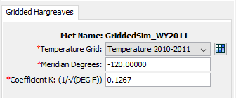
Figure 7. Component editor for the gridded Hargreaves shortwave method.

Gridded Shortwave

The gridded shortwave method is designed to work with the ModClark gridded transform. However, it can be used with other area-average transform methods as well. The most common use of the method is to utilize gridded shortwave radiation estimates produced by an external model, for example, a dynamic atmospheric model. If it is used with a transform method other than ModClark, an area-weighted average of the grid cells in the subbasin is used to compute the shortwave radiation time-series for each subbasin.

The gridded shortwave method includes a Component Editor with parameter data for all subbasins in the meteorologic model. The Watershed Explorer provides access to the shortwave component editor using a picture of solar radiation (Figure 6).

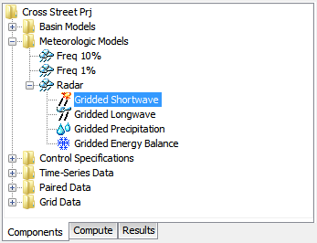
Figure 6. A meteorologic model using the gridded shortwave method with a component editor for all subbasins in the meteorologic model.

A Component Editor for all subbasins in the meteorologic model includes the selection of the data source (Figure 7). A radiation gridset must be selected for all subbasins. The current gridsets are shown in the selection list. If there are many different gridsets available, you may wish to choose a gridset from the selector accessed with the grid button next to the selection list. The selector displays the description for each gridset, making it easier to select the correct one.

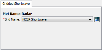
Figure 7. Specifying the shortwave radiation data source for the gridded shortwave method.

Hargreaves

The Hargreaves shortwave method implements the shortwave radiation algorithm described by Hargreaves and Samani (1982). The method calculates the solar declination and solar angle for each time interval of the simulation, using the coordinates of the subbasin, Julian day of the year, and time at the middle of the compute interval. The solar values are used to compute the extra-terrestrial radiation for each subbasin. The daily temperature range, daily maximum temperature less daily minimum temperature, functions as a proxy for cloud cover. Shortwave radiation arriving at the ground surface is computed as a function of extraterrestrial radiation and the daily temperature range.

The Hargreaves shortwave method is parameterized for all subbasins in the basin model. Select the Hargreaves shortwave node in the Watershed Explorer (Figure 8) to access the Hargreaves shortwave Component Editor (Figure 9). An air temperature gage must be selected in the atmospheric variables for each subbasin. The temperature gage should have sub-daily measurements so that daily minimum and maximum temperatures can be analyzed. The subbasin atmospheric variables Component Editor is accessed by clicking on a subbasins node in Watershed Explorer.

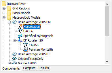
Figure 8. A meteorologic model using the Hargreaves shortwave radiation method with a component editor for the basin.

The Hargreaves shortwave Component Editor is shown in Figure 9. The user must enter the central meridian of the time zone and the Hargreaves shortwave coefficient. If the basin model spans multiple time zones, then enter the central meridian for the time zone containing most of the basin model drainage area. The central meridian is the longitude at the center of the local time zone. Meridians west of zero longitude should be specified as negative while meridians east of zero longitude should be specified as positive. The meridian may be specified in decimal degrees or degrees, minutes, and seconds depending on the program settings. The default Hargreaves shortwave coefficient is 0.17 per square root of degrees Celsius; this is equivalent to 0.1267 per square root of degrees Fahrenheit. The default Hargreaves shortwave coefficient of 0.17 per square root of degree Celcsus is implicit in the Hargreaves and Samani (1985) potential evapotranspiration formulation. The Hargreaves shortwave coefficient can be adjusted by the user.

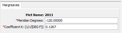
Figure 9. Entering the longitude of the central meridian of the local time zone (US Pacific in this case) and Hargreaves shortwave radiation coefficient.

Specified Pyranograph

A pyranometer is an instrument that can measure incoming solar shortwave radiation. They are not part of basic meteorological observation stations, but may be included at first order stations. This method may be used to import observed values from a pyranometer or it may be used to import estimates produced by an external model. This is the recommended choice for use with the Priestley Taylor evapotranspiration method, where an effective radiation is used which includes both shortwave and longwave radiation.

The specified pyranograph method includes a Component Editor with parameter data for all subbasins in the meteorologic model. The Watershed Explorer provides access to the shortwave component editors using a picture of solar radiation (Figure 10).

The Component Editor for all subbasins in the meteorologic model includes the time-series gage of shortwave radiation for each subbasin (Figure 11). A solar radiation gage must be selected for a subbasin. The current gages are shown in the selection list.

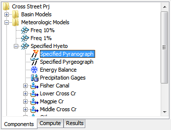
Figure 10. A meteorologic model using the specified pyranograph shortwave method with a component editor for all subbasins.

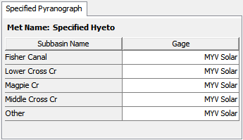
Figure 11. Specifying the shortwave radiation time-series gage for each subbasin.