Uncertainty assessment is the process of determining the total error in the simulated watershed response, for example, the flow at the outlet. The simulated flow at the outlet actually depends on many individual components each with its own error. There is error in the meteorologic data because it is generally impossible to accurately measure precipitation at the same spatial and temporal scale as the land surface processes. There is error in the models of the hydrologic processes because it is generally impossible to include every possible process at the scale it occurs, for example, animal burrows or plant transpiration. There is error in the model parameter values because the equations are solved at a scale ranging from meters up to whole subbasins and area-average values must be used. The error in the whole watershed response includes all of these individual errors and the complex way in which they interact.

The watershed model is very complex and it may not be possible to attribute the total error to individual components. An error in the precipitation data may be compensated with a corresponding error in the infiltration parameter values. An error in the mathematical formulation of the infiltration or transpiration process may be compensated with a corresponding error in the parameter values. An assumption about process scale may lead to effective area-averaged parameter values that do not match values that would be measured in the field. It is usually not possible to determine the exact error in each component or how the errors are interacting and accumulating throughout the watershed model.

The error in an individual model parameter may be described with a probability distribution during an uncertainty assessment. In one case the selected process model is well-suited to the watershed, the input to the model is accurate, and the parameters can be estimated from field observations. In this first case there is very little uncertainty in the parameter value. In another case the model is missing important subtleties of the physical process, the input is poor, and parameter estimation is difficult. In this second case there is a high degree of uncertainty in the parameter value. In both cases, a probability distribution can be parameterized to reflect the uncertainty in the parameter, either small or large. Different model parameters require differently formulated probability distributions and they may change from one watershed to another or from one historical time period to another.

The Monte Carlo method is one approach to estimating the uncertainty in the simulated watershed response given the uncertainty in each of the model parameters. The Monte Carlo method works by creating many alternative models of the watershed using an automated sampling procedure. Each sample is created by sampling the model parameters according to their individual probability distribution. Each sample is simulated to obtain a watershed response corresponding to the sampled parameter values. All of the responses from all of the samples can be analyzed statistically to evaluate the uncertainty in the simulated watershed response. The program uses the Monte Carlo method to perform the uncertainty assessment.

Within HEC-HMS, uncertainty analyses are one of the simulation components that can compute results. Each analysis is composed of a basin model, meteorologic model, and time control information. The analysis also includes a selection of parameters to be evaluated and a description of the uncertainty for each parameter. Several options are provided for how the uncertainty is described for each parameter. A variety of results graphs are available from the Watershed Explorer for assessing the uncertainty in simulated watershed response.

The uncertainty analysis primarily addresses the uncertainty in hydrologic model parameters which may be due to incorrect parameter estimation, scale, or other problems. The user must identify each uncertain parameter during the assessment and describe the uncertainty using an appropriate probability distribution. Uncertainty in the meteorologic data is not specifically addressed within the program. Evaluation of uncertainty in meteorology must be carried out using an assessment framework that integrates meteorologic and hydrologic uncertainty. The Watershed Analysis Tool (HEC-WAT) modeling framework to be capable of carrying out such an integrated assessment. The uncertainty analysis in HEC-HMS is designed to work with HEC-WAT with expanded integration capabilities planned for future releases.

Creating a New Uncertainty Analysis

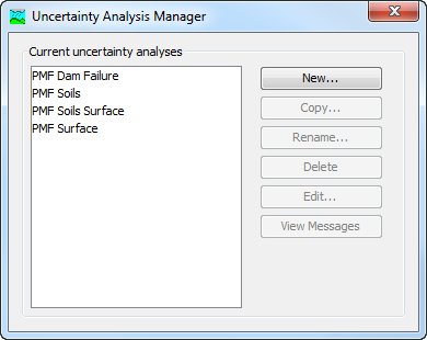
A new uncertainty analysis is created using a wizard that helps you navigate the steps to creating a new analysis. There are two ways to access the wizard. The first way to access the wizard is to click on the Compute menu and select the Create Compute | Uncertainty Analysis command; it is only enabled if at least one basin model and meteorologic model exist. The wizard will open and begin the process of creating a new uncertainty analysis. The second way to access the wizard is from the Uncertainty Analysis Manager. Click on the Compute menu and select the Uncertainty Analysis Manager command. The Uncertainty Analysis Manager will open and show any analyses that already exist. Press the New… button to access the wizard and begin the process of creating an uncertainty analysis, as shown in Figure 1.

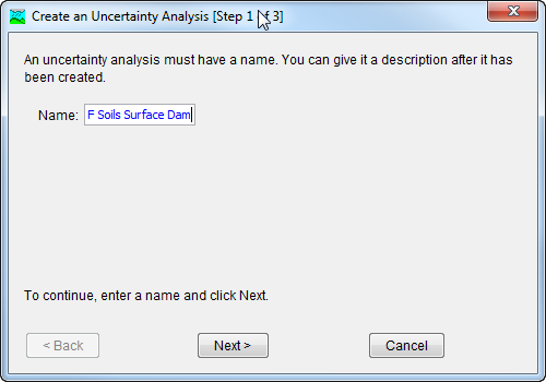
Figure 1. Beginning the process of creating a new uncertainty analysis using the Uncertainty Analysis Manager.
The first step of creating an uncertainty analysis is to provide the name for the new analysis (Figure 2). A default name is provided for the new uncertainty analysis; you can use the default or replace it with your own choice. After you finish creating the analysis you can add a description to it. If you change your mind and do not want to create a new uncertainty analysis, you can press the Cancel button at the bottom of the wizard or the X button in the upper right corner of the wizard. The Cancel button can be pressed at any time you are using the wizard. Press the Next> button when you are satisfied with the name you have entered and are ready to proceed to the next step.

Figure 2. Entering a name for a new uncertainty analysis. The remaining steps are to select a basin model and a meteorologic model.
The second step of creating an uncertainty analysis is to select a basin model. All of the basin models that are currently part of the project are displayed in alphabetical order. By default the first basin model in the table is selected. The selected basin model is highlighted. You can use your mouse to select a different basin model by clicking on it in the table of available choices. You can also use the arrow keys on your keyboard to select a different basin model. Press the Next> button when you are satisfied with the basin model you have selected and are ready to proceed to the next step. Press the <Back button if you wish to return to the previous step and change the name for the new uncertainty analysis.

The third step of creating an uncertainty analysis is to select a meteorologic model. All of the meteorologic models that are currently part of the project are displayed in alphabetical order. By default the first meteorologic model in the table is selected. The selected meteorologic model is highlighted. You can use your mouse to select a different meteorologic model by clicking on it in the table of available choices. You can also use the arrow keys on your keyboard to select a different meteorologic model. You are responsible for selecting a basin model in step two and a meteorologic model in this step that will successfully combine to compute results. Press the Finish button when you are satisfied with the name you have entered, the basin model and meteorologic model you selected, and are ready to create the uncertainty analysis. Press the <Back button if you wish to return to the previous step and select a different basin model.

Copying an Uncertainty Analysis

There are two ways to copy an uncertainty analysis. Both methods for copying an analysis create an exact duplicate with a different name. Once the copy has been made it is independent of the original and they do not interact.

The first way to create a copy is to use the Uncertainty Analysis Manager, which is accessed from the Compute menu. Select the uncertainty analysis you wish to copy by clicking on it in the list of current uncertainty analyses. The selected analysis is highlighted after you select it. After you select an analysis you can press the Copy… button on the right side of the window. The Copy Uncertainty Analysis window (Figure 3) will open where you can name and describe the copy that will be created. A default name is provided for the copy; you can use the default or replace it with your own choice. A description can also be entered; if it is long you can use the button to the right of the description field to open an editor. When you are satisfied with the name and description, press the Copy button to finish the process of copying the selected uncertainty analysis. You cannot press the Copy button if no name is specified. If you change your mind and do not want to copy the selected uncertainty analysis, press the Cancel button or the X button in the upper right to return to the Uncertainty Analysis Manager window.

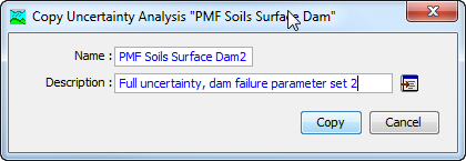
Figure 3. Creating a copy of an uncertainty analysis.

The second way to copy is from the "Compute" tab of the Watershed Explorer. Move the mouse over the uncertainty analysis you wish to copy and press the right mouse button (Figure 4) A context menu is displayed that contains several choices including copy. Click the Create Copy… command. The Copy Uncertainty Analysis window will open where you can name and describe the copy that will be created. A default name is provided for the copy; you can use the default or replace it with your own choice. A description can also be entered; if it is long you can use the button to the right of the description field to open an editor. When you are satisfied with the name and description, press the Copy button to finish the process of copying the selected uncertainty analysis. You cannot press the Copy button if no name is specified. If you change your mind and do not want to copy the selected uncertainty analysis, press the Cancel button or the X button in the upper right of the Copy Uncertainty Analysis window to return to the Watershed Explorer.

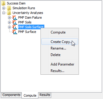
Figure 4. Copying an uncertainty analysis from the Watershed Explorer. The Copy Uncertainty Analysis window will appear after the Create Copy menu command is selected.

Renaming an Uncertainty Analysis

There are two ways to rename an uncertainty analysis. Both methods for renaming an analysis change its name and perform other necessary operations.

The first way to perform a rename is to use the Uncertainty Analysis Manager, which you can access from the Compute menu. Select the uncertainty analysis you wish to rename by clicking on it in the list of current analyses. The selected analysis is highlighted after you select it. After you select an analysis you can press the Rename… button on the right side of the window. The Rename Uncertainty Analysis window (Figure 5) will open where you can provide the new name. If you wish you can also change the description at the same time. If the new description will be long, you can use the button to the right of the description field to open an editor. When you are satisfied with the name and description, press the Rename button to finish the process of renaming the selected uncertainty analysis. You cannot press the Rename button if no name is specified. If you change your mind and do not want to rename the selected uncertainty analysis, press the Cancel button or the X button in the upper right of the Rename Uncertainty Analysis window to return to the Uncertainty Analysis Manager window.

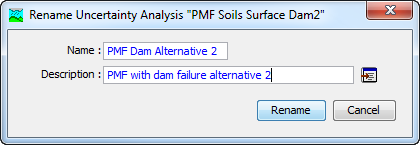
Figure 5. Renaming an uncertainty analysis. This was accessed from the Uncertainty Analysis Manager.

The second way to rename is from the "Compute" tab of the Watershed Explorer. Select the uncertainty analysis you wish to rename by clicking on it in the Watershed Explorer; it will become highlighted. Keep the mouse over the selected analysis and click the left mouse button again. The highlighted name will change to editing mode (Figure 6). You can then move the cursor with the arrow keys on the keyboard or by clicking with the mouse. You can also use the mouse to select some or all of the name. Change the name by typing with the keyboard. When you have finished changing the name, press the Enter key to finalize your choice. You can also finalize your choice by clicking elsewhere on the "Compute" tab. If you change your mind while in editing mode and do not want to rename the selected uncertainty analysis, press the Escape key.

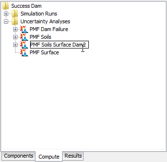
Figure 6. Renaming an uncertainty analysis in the Watershed Explorer.

Deleting an Uncertainty Analysis

There are two ways to delete an uncertainty analysis. Both methods for deleting an analysis remove it from the project and automatically delete previously computed results. Once an analysis has been deleted it cannot be retrieved or undeleted.

The first way to perform a deletion is to use the Uncertainty Analysis Manager, which you can access from the Compute menu. Select the uncertainty analysis you wish to delete by clicking on it in the list of current analyses. The selected analysis is highlighted after you select it. After you select an analysis you can press the Delete button on the right side of the window. A window will open where you must confirm that you wish to delete the selected analysis as shown in Figure 7. Press the OK button to delete the analysis. If you change your mind and do not want to delete the selected uncertainty analysis, press the Cancel button or the X button in the upper right to return to the Uncertainty Analysis Manager window.

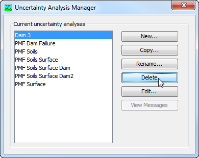
Figure 7. Preparing to delete an uncertainty analysis from the Uncertainty Analysis Manager. A confirmation will be required after pressing the Delete button.

The second way to delete is from the "Compute" tab of the Watershed Explorer. Select the uncertainty analysis you wish to delete by clicking on it in the Watershed Explorer; it will become highlighted (Figure 8). Keep the mouse over the selected analysis and click the right mouse button. A context menu is displayed that contains several choices including delete. Click the Delete command. A window will open where you must confirm that you wish to delete the selected analysis. Press the OK button to delete the analysis. If you change your mind and do not want to delete the selected uncertainty analysis, press the Cancel button or the X button in the upper right to return to the Watershed Explorer.

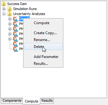
Figure 8. Deleting an uncertainty analysis in the Watershed Explorer.

Selecting Components

One of the principal tasks when creating an uncertainty analysis using the wizard is the selection of the components that will be used to compute uncertainty results. The components include the basin model and the meteorologic model. These components are selected when creating a new uncertainty analysis with the wizard. However, you can change the basin model and meteorologic model you wish to use at any time using the Component Editor for the uncertainty analysis. Access the Component Editor from the "Compute" tab of the Watershed Explorer (Figure 9). If necessary, click on the "Uncertainty Analyses" folder to expand it and view the available uncertainty analyses. The Component Editor contains a basin model selection list that includes all of the basin models in the project. The Component Editor also contains a meteorologic model selection list that includes all of the meteorologic models in the project.

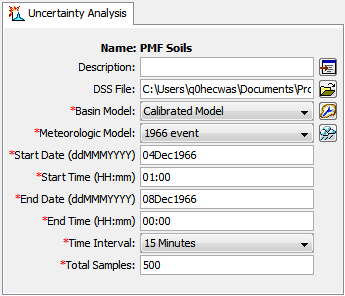
Figure 9. The uncertainty analysis component editor can be used to change the selected components, time window, and total number of samples.

Entering a Time Window

You must enter a start date and time and an end date and time for the uncertainty analysis. The time control information is not specified in the wizard used to create the uncertainty analysis. The time control information must be entered after the analysis is created using the Component Editor for the uncertainty analysis (Figure 9). Enter the start date using the indicated format for numeric day, abbreviated month, and four-digit year. Enter the end date using the same format. The start time and end time are entered using a 24-hour time format. Choose a time interval from the available options which range from 1 minute up to 1 day. Finally, the start time and end time must each be an integer number of time intervals after the beginning of the day.

Total Samples and Convergence

You must enter the total number of samples for the uncertainty analysis. The number of samples is not specified in the wizard used to create the uncertainty analysis. The total samples must be entered after the analysis is created using the Component Editor for the uncertainty analysis (Figure 9). The number of samples specifies how many times the model parameters will be sampled during the uncertainty assessment.

The total number of samples must be large enough to accurately estimate the uncertainty in the watershed response. The process of determining when the watershed response has been accurately estimated is called convergence. Convergence is achieved when statistical measures of the watershed response do not change if more samples are computed. For example, one watershed response that is often considered is the maximum pool elevation in a reservoir. The maximum pool elevation can be recorded for each sample and the mean value can be computed over all samples. Convergence in the mean maximum pool elevation is achieved when increasing the number of samples does not result in a change in the computed mean. If the standard deviation in the maximum pool elevation were considered, then additional samples would have to be computed until the computed standard deviation did not change. Fewer samples are required to estimate the mean watershed response compared to the standard deviation in the response.

The user must select an appropriate number of samples to compute for the uncertainty analysis. The number of samples required to achieve convergence depends on many factors including how a watershed is modeled as well as which watershed response statistics are considered. Automatic convergence criteria are not available at this time but are planned for a future release.

Adding and Deleting Parameters

The parameters that will be sampled during the uncertainty assessment may be at any subbasin, reach, or reservoir element in the basin model. Parameters that can be chosen for sampling are a selected set of the canopy, surface, lossrate, transform, and baseflow parameters in the subbasin element. Selected parameters can also be chosen for sampling from the routing parameters in the reach and from the components in the reservoir. Two types of parameters can be selected for sampling. The first type includes parameters in conceptual models such as the time of concentration for a unit hydrograph. The second type includes parameters in physically-based models subject to scaling issues, such as soil hydraulic conductivity or channel bottom width. Most parameters in the basin model can be classified as one of these two types.

Add a new parameter to an uncertainty analysis using the Watershed Explorer. Move the mouse over the analysis and press the right mouse button (Figure 10). A context menu is displayed that contains several choices including adding a parameter. Click the Add Parameter command. The parameters are automatically named and numbered beginning with "Parameter 1" and increasing the number as more parameters are added.

Meteorologic model parameters that can be added are shown in Table 1. The subbasin canopy parameters that can be added are shown in Table 2. Subbasin surface parameters that can be added are shown in Table 3 and loss rate parameters are shown in Table 4. The available subbasin transform parameters are shown in Table 5 and baseflow parameters are shown in Table 6. Reach routing parameters that can be added are shown in Table 7 while available reservoir parameters that can be added are shown in Table 8.
Delete a parameter from an uncertainty analysis using the Watershed Explorer. Select the parameter you wish to delete by clicking on it in the Watershed Explorer; it will become highlighted. Keep the mouse over the selected parameter and click the right mouse button (Figure 11). A context menu is displayed that contains several choices including deleting a parameter. Click the Delete Parameter command.

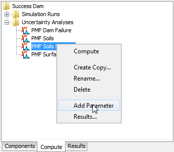
Figure 10. Adding a parameter to an uncertainty analysis.

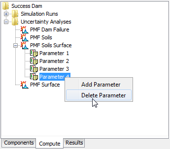
Figure 11. Deleting a selected parameter from an uncertainty analysis.

Table 1.Meteorologic model parameters available for sampling.

Method	Parameter
HMR52 Precipitation	X Coordinate
	Y Coordinate
	Storm Area
	Storm Orientation
	Peak Hour
Hypothetical Precipitation	Storm Depth
	Storm Temporal Pattern
	Depth-Area Reduction Function
Specified Precipitation	Total Depth
Temperature Index Snow	Wet Melt Rate
	Lapse Rate
	Initial Snow Water Equivalent

Table 2. Subbasin canopy parameters available for sampling.

Method	Parameter
Dynamic	Initial Storage
Gridded Simple	Initial Storage
Simple	Initial Storage
	Maximum Storage

Table 3. Subbasin surface parameters available for sampling.

Method	Parameter
Gridded Simple	Initial Storage
Simple	Initial Storage
	Maximum Storage

Table 4. Subbasin lossrate parameters available for sampling.

Method	Parameter
Curve Number	Initial Abstraction
	Constant Rate
	Impervious Area
Deficit Constant	Initial Deficit
	Maximum Deficit
	Constant Rate
	Impervious Area
Exponential	Initial Range
	Initial Coefficient
	Coefficient Ratio
	Exponent
	Impervious Area
Green Ampt	Initial Content Saturated Content
	Suction
	Conductivity
	Impervious Area
Gridded Curve Number	Initial Abstraction Ratio
	Potential Retention Scale Factor
Gridded Deficit Constant	Initial Deficit Ratio
	Maximum Deficit Ratio
	Constant Rate Ratio
	Impervious Area Ratio
Gridded SMA	Soil Initial Storage
	Groundwater 1 and 2 Initial Storage
Initial Constant	Initial Loss
	Constant Rate
	Impervious Area
Smith Parlange	Initial Content
	Residual Content
	Saturated Content
	Bubbling Pressure
	Pore Distribution
	Conductivity
	Beta Zero
	Impervious Area
Soil Moisture Accounting	Soil Initial Storage
	Soil Storage
	Soil Tension Storage
	Soil Tension Storage
	Soil Percolation
	Groundwater 1 and 2 Initial Storage
	Groundwater 1 and 2 Storage
	Groundwater 1 and 2 Percolation
	Groundwater 1 and 2 Coefficient
	Impervious Area

Table 5. Subbasin transform parameters available for sampling.

Method	Parameter
Clark	Time of Concentration
	Storage Coefficient
Kinematic	Plane Length
Wave	Plane Slope
	Plane Roughness
	Subcollector, Collector, and Main Channel Length
	Subcollector, Collector, and Main Channel Slope
	Subcollector, Collector, and Main Channel Manning's n
	Subcollector, Collector, and Main Channel Bottom Width ¹
	Subcollector, Collector, and Main Channel Side Slope ²
ModClark	Time of Concentration
	Storage Coefficient
SCS	Time Lag
S-Graph	Time Lag
Snyder	Peaking Coefficient
	Standard Lag
1. Bottom width can be selected for cross section shapes: deep, rectangle, trapezoid.
2. Side slope can be selected for cross section shapes: trapezoid, triangle.

Table 6. Subbasin baseflow parameters available for sampling.

Method	Parameter
Bounded Recession	Initial Flow Rate or Initial Flow Rate per Area ¹
	Recession Constant
Linear Reservoir	GW 1 and 2 Initial Flow Rate or Initial Flow Rate per Area ¹
	Groundwater 1 and 2 Storage Coefficient
	Groundwater 1 and 2 Number of Steps
Nonlinear Boussinesq	Initial Flow Rate or Initial Flow Rate per Area ¹
	Characteristic Length
	Hydraulic Conductivity
	Drainable Porosity
	Threshold Ratio or Threshold Flow Rate ²
Recession	Initial Flow Rate or Initial Flow Rate per Area ¹
	Recession Constant
	Threshold Ratio or Threshold Flow Rate ²
1. The available parameter depends on the method selected for specifying the initial condition.
2. The available parameter depends on the method selected for specifying the recession threshold.

Table 7. Reach routing parameters available for sampling.

Method	Parameter
Kinematic Wave	Initial Outflow
	Energy Slope
	Manning's n
	Diameter ¹
	Bottom Width ²
	Side Slope ³
Lag	Initial Outflow
	Lag
Modified Puls	Initial Outflow
	Subreaches
Muskingum	Initial Outflow
	K
	X
	Subreaches
Muskingum Cunge	Initial Outflow
	Energy Slope
	Manning's n
	Diameter ¹
	Bottom Width ²
	Side Slope ³
Normal Depth	Initial Outflow
	Energy Slope
	Manning's n
	Diameter ¹
	Bottom Width ²
	Side Slope ³
Straddle Stager	Initial Outflow
	Lag
	Duration
1. Available for the circle cross section.
2. Available for deep, rectangle, and trapezoid cross section.
3. Available for trapezoid and triangle cross section.

Table 8. Reservoir parameters available for sampling.

Method	Parameter
Initial Condition	Initial Elevation ¹
	Initial Outflow ¹
	Initial Storage ¹
Orifice Outlet	Coefficient
Culvert	Entrance Coefficient
	Exit Coefficient
	Manning's n
Level Dam Top	Coefficient
Broadcrested Spillway	Coefficient
Overtop Breach	Top Elevation
	Bottom Elevation
	Bottom Width
	Left Side Slope
	Right Side Slope
	Development Time
Piping Breach	Top Elevation
	Bottom Elevation
	Piping Elevation
	Bottom Width
	Left Side Slope
	Right Side Slope
	Piping Coefficient
	Development Time
1. The available parameter depends on the method selected for specifying the initial condition.
Nonlevel Dam Top	Coefficient

Specifying Parameter Information

Information must be specified for each selected parameter. The first selection is the element (Figure 12). The element selection list includes all of the elements in the basin model where at least one parameter is available for selection. The parameters available for selection will depend on the methods that have been selected. Once the element has been selected, the second selection is the parameter at the chosen element. All of the available parameters at the selected element are included in the list. If the element selection is changed, then a new parameter selection will also need to be made.

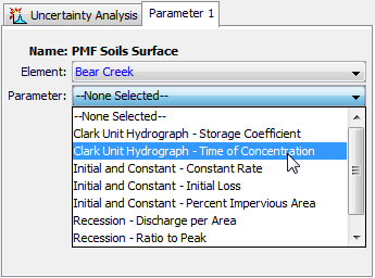
Figure 12. Choosing an element where a parameter will be sampled, and selecting the parameter at that element.

There are four different methods for sampling the selected parameter. The Component Editor will display the appropriate property information depending on the sampling method that you choose. The Simple Distribution sampling method allows you to choose a probability distribution and then samples the parameter independently of all other parameters selected in the uncertainty analysis. The Monthly Distribution sampling method allows you to choose an analytical probability distribution and enter unique distribution properties for each month; the parameter is sampled independently of all other parameters in the analysis. The Regression With Additive Error sampling method allows you to choose a previously selected parameter and then define a linear relationship between this dependent parameter and the previously selected parameter; an epsilon error term can be added to the linear relationship. The Specified Values sampling method allows the user to specify a paired data curve for each of the selected parameters. The program will systematically go through the list of parameter values when sampling values for the uncertainty analysis. If multiple parameters are selected, then the same row from the parameter value paired data tables will be selected during a parameter sample. This sampling method was designed to use results from an MCMC optimization trial. The information specified for each of the four sampling methods is explained in the following sections.

Simple Distribution

The Simple Distribution sampling method can be used to define the uncertainty in a parameter independently of all other parameters in the analysis. The sampling process is defined by the selection of a probability distribution. There are eight analytical functions available with the choices shown in Table 9. There is also the option of choosing an empirical function ("User-Specified"). The empirical function must be defined in the paired data manager as a Cumulative Probability Distribution before it can be selected in the sampling method. A new parameter value is sampled for each iteration of the analysis, with draws coming from the specified probability distribution and distribution parameters.

The selection of a probability distribution determines which additional parameters must be entered. An example of the Component Editor is shown in Figure 13. Several of the distributions have a minimum value of zero, but may need to be applied with parameters that typically begin their range at a value greater than zero. A shift parameter is included with these functions for this purpose.

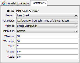
Figure 13. Setting sampling properties for a parameter using the Simple Distribution method.

All of the available distribution choices include a minimum and maximum value. These limits are imposed as constraints on the parameter sampling process. If the value computed for a sample falls below the minimum or above the maximum, then a new value is sampled. This process is repeated until a sampled parameter value is generated that falls between the minimum and maximum, which effectively truncates the distribution. These constraints are separate from the mathematical features of the selected distribution. The limits are useful for enforcing physical process limitations or restricting the sampling to a reasonable range for the selected parameter.

Monthly Distribution

The Monthly Distribution sampling method can be used to define the uncertainty in a parameter that shows seasonal variation. The sampling process is defined by the selection of a probability distribution along with separate distribution parameter values for each month. The eight available choices of probability distribution are shown in Table 9. A new parameter value is sampled from the specified probability distribution for each iteration in the analysis. The simulation start date and time of the uncertainty analysis will be used to determine which monthly distribution parameter will be used in the sampling process.

Table 9. Analytical probability distribution functions available for parameter sampling and epsilon error term sampling. Parameter labels used in the program are shown below the formula.

Function	Formula
Beta	$\begin{array}{l}f(x)=\frac{1}{B(\alpha,\beta)}\frac{(x-lower)^{\alpha-1}(upper-x)^{\beta-1}}{(upper-lower)^{\alpha+\beta-1}}\end{array}$
	$\begin{array}{l}B(\alpha,\beta)\end{array}$ is the Beta function
Exponential	$\begin{array}{l}f(x)=\frac{1}{\mu}\exp(-\frac{x-shift}{\mu})\end{array}$
Gamma	$\begin{array}{l}f(x)=\frac{(x-shift)^{\alpha-1}}{\beta^{\alpha}}\frac{1}{\Gamma(\alpha)}\exp(-\frac{x-min}{\beta})\end{array}$
	Shape=α, Scale=β
	$\begin{array}{l}\Gamma(\alpha)\end{array}$ is the Gamma function
Gumbel	$\begin{array}{l}f(x)=\frac{1}{\alpha}\exp(-(\frac{x-\xi}{\alpha}+\exp(-\frac{x-\xi}{\alpha})))\end{array}$
	Location = ξ, Scale = α
Log-normal	$\begin{array}{l}f(x)=\frac{1}{x\sqrt{2\pi\sigma^{2}}}\exp(-\frac{(\log(x)-\mu)^{2}}{2\sigma^{2}})\end{array}$
Normal	$\begin{array}{l}f(x)=\frac{1}{\sqrt{2\pi\sigma^{2}}}\exp(-\frac{(x-\mu)^{2}}{2\sigma^{2}})\end{array}$
Triangular	$\begin{array}{l}f(x)=\begin{cases} 0, & x < a,\\ \frac{2(x-a)}{(b-a)(c-a)}, & a \le x < c,\\ \frac{2}{b-a}, & x = c,\\ \frac{2(b-x)}{(b-a)(b-c)}, & c < x \le b,\\ 0, & b < x. \end{cases}\end{array}$
	Lower = a, Upper = b, Mode = c
Uniform	$\begin{array}{l}f(x)=\begin{cases} \frac{1}{b-a}, & x \in [a,b] \\ 0, & \text{otherwise}. \end{cases}\end{array}$
	Lower=a, Upper=b
Weibull	$\begin{array}{l}f(x)=\begin{cases} \frac{k}{\lambda}(\frac{x-shift}{\lambda})^{k-1}\exp(-(\frac{x-shift}{\lambda})^{k}), & x \ge 0 \\ 0, & x < 0 \end{cases}\end{array}$
	Shape=k, Scale=λ

The selection of a probability distribution determines which additional parameters must be entered. An example of the Component Editor is shown in Figure 14. A table is used to enter the probability distribution parameter values for each month. A shift parameter is included with probability distribution functions that begin at zero to account for parameters that for physical reasons should begin at a value greater than zero.

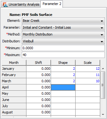
Figure 14. Setting sampling properties for a parameter using the Monthly Distribution method.

All of the available probability distribution choices include minimum and maximum limits that are imposed on the parameter sampling process. The parameter will be repeatedly sampled until a value is obtained that falls between the minimum and maximum, which effectively truncates the probability distribution. These constraints are separate from the mathematical features of the selected probability distribution. The limits are useful for enforcing physical process limitations or restricting the sampling to a reasonable range for the selected parameter. The same minimum and maximum is used for all months of the year.

Regression With Additive Error

The Regression With Additive Error sampling method can be used to define the uncertainty in a parameter that has a dependency linkage to another parameter in the analysis. The sampling process is defined by selecting an independent parameter which will become the basis for generating the sampled value at this parameter. In order for a regression element to be selected, a parameter with an independent sampling method (i.e., simple distribution, monthly distribution or specified parameters) must be created first. A regression relationship is defined between the two parameters. The calculation process proceeds for a sample by first accessing the value computed for the independent parameter. Then the regression is applied to calculate the preliminary parameter value for this parameter. An epsilon error term is then calculated using one of the eight available probability distribution choices (Table 9). The sampled epsilon error is added to the preliminary parameter value to produce the value used for a sample. From sample to sample, the values that vary are the sampled value for the independent regression parameter and the error term. For realization of regression parameter x_i, user-specified slope m, user-specified intercept b and value sampled from the specified error distribution ε_i, the sampled parameter value Y_i is:

A regression element, "Reg Element," must be selected as shown in the Component Editor (Figure 15). The available choices will be taken from the parameters that have been previously defined in the uncertainty analysis. Once a regression element is selected, the regression parameter in the regression element can be selected. The parameter choices will include all of the parameters in the uncertainty analysis at the selected regression element.

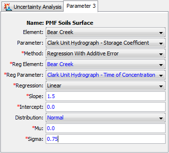
Figure 15. Setting sampling properties for a parameter using the Dependent Plus Error method.

A relationship is used to define the linkage from the selected regression parameter to this parameter. The first possibility for the relationship is a linear one. Alternatively, a semi-logarithmic relationship may be selected. In both cases, you must enter the slope and intercept for the relationship. If the linear relationship is selected, the slope and intercept values should be appropriate for "normal" space. If the log-linear relationship is selected, the slope and intercept values should be appropriate for "natural logarithmic" space.

An epsilon error term is added to the preliminary parameter value calculated from the regression parameter and the linear or semi-logarithmic relationship. The epsilon term represents the error in the fitting relationship between the regression parameter and this parameter. You may choose any one of the eight analytical probability distributions to represent the error term. Based on the selected distribution, parameter coefficients must be entered to define the distribution.

Specified Values

The Specified Values sampling method allows the user to specify one or more sequences of parameter values via a Parameter Value Samples Paired Data record. The paired data records can be created using the paired data component manager. Figure 16 shows the Component Editor for a Parameter Value Samples Paired Data record. The primary use for this sampling method is to allow a user to sample parameter values previously generated using a stochastic optimization scheme like Markov Chain Monte Carlo. However, any means for generating a parameter set may be employed.

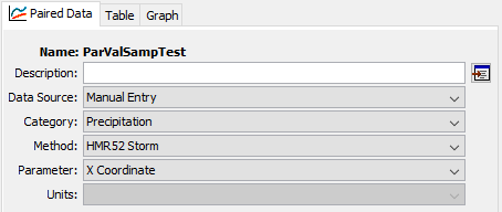
Figure 16. Default settings for a new Parameter Value Samples Paired Data record.

A Parameter Value Sample Paired Data record can be used in an Uncertainty Analysis by selecting the Specified Values method for the uncertainty analysis method and selecting the Paired Data record for the Parameter Value (Figure 17). The Uncertainty Analysis editor will allow the user to select any Parameter Value Sample Paired Data record; however, if a record with a mismatched parameter is used, then an error will be thrown at compute informing the user that the parameter type is not an appropriate match. For example, trying to use a Paired Data record for Initial Deficit values when sampling Time of Concentration will produce an error. An error will also result if the Paired Data record does not contain any entries. The Paired Data record can be any length relative to the selected number of total samples for the uncertainty analysis: if the Paired Data record is shorter, then the list of parameters will be recycled until the requisite number of samples is met; if it is longer, then not all values will be sampled.

Figure 17. Specified Values Uncertainty Analysis set up with a Parameter Value Paired Data record.

Sampling of parameter values proceeds index-wise. If more than one parameter is varied using this method, then samples will follow the order of parameters contained in all of the Paired Data records (i.e. index 1 for all parameters, then index 2 if it exists, and so on). If one record is shorter than another, then it will begin recycling values before the other parameters.

When maintaining correlation between parameters is desired, such as when applying sampled parameter sets generated using Markov Chain Monte Carlo, then each row of each Parameter Value Paired Data record is intended to represent a single set of parameters. The intention is that the relationship between parameters is maintained to reflect the correlation between variables as estimated by the MCMC procedure. Often two or more different parameters will have opposite or canceling effects on the goodness-of-fit, so it is more likely that they will be sampled in a manner that reflects this variability.

If the user wishes to use parameter sets generated by a Markov Chain Monte Carlo Optimization Trial, then the Parameter Sample Creator, available in the Tools menu after running the Optimization Trial (see Figure 18), can help.

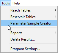
Figure 18. Accessing the Parameter Sample Creator tool

In the Parameter Sample Creator dialog, the available MCMC Optimization Trials are shown (Figure 19). If the user highlights one and selects Create…, the user is prompted to enter a name and a description. Once created, the set of Parameter Value Sample Paired Data Records is available for use in an Uncertainty Analysis with the Specified Values sampling method.

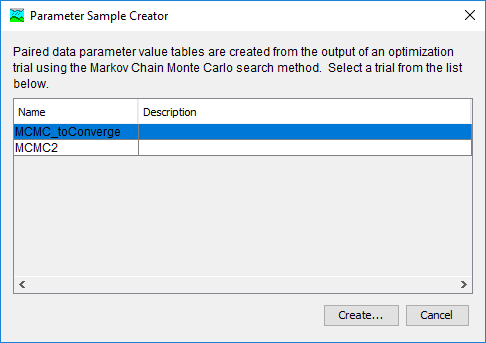
Figure 19. Parameter Sample Creator dialog box with available MCMC Optimization Trials for selection.