A subbasin element represents a catchment where precipitation falls and causes surface runoff. Erosion within the catchment will result from a combination of several different physical processes including post-fire conditions. Rain drops cause erosion when they impact the ground surface and break apart the top layer of the soil, dislodging soil particles to move with the overland flow. Overland flow also imparts an erosive energy to the ground surface that may further break apart the top soil layer. As the overland flow rate increases, the flow becomes concentrated in rills which focuses erosive energy and further erodes the surface. Total erosion is closely linked to precipitation rate, land surface slope, and condition of the surface. In some cases, soil eroded high in the catchment may deposit before reaching the outlet of the subbasin.

Certain simulation features are common to all of the surface erosion methods available for the subbasin element. Each erosion method computes the total sediment load transported out of the subbasin during a storm. This calculation process is repeated for each storm during the simulation time window. The sediment load must be distributed into a time-series of sediment discharge from the subbasin. The distribution of sediment is based on the computed hydrograph and the power function approach of Haan et al. (1994). The power function is given by:

where c_t is the sediment concentration at time t, kⁱ is the proportion of the load for the current event i to the total annual load, Q_t is the subbasin discharge (flowrate) at time t, and a is an exponent entered by the user.

Also common to all of the surface erosion methods is the approach to grain size distribution. All of the methods first compute the bulk sediment discharge which includes all grain sizes. A gradation curve specifies the proportion of the total sediment discharge that should be apportioned to each grain size class or subclass. A gradation curve must be defined by the user and selected at each subbasin. A different gradation curve can be used at each subbasin to represent differences in the erosion, deposition, and resuspension processes within each subbasin. The combination of these processes is often represented by an enrichment ratio.

Selecting an Erosion Method

The erosion method for a subbasin is selected on the Component Editor for the subbasin element (Figure 1). Access the Component Editor by clicking the subbasin element icon on the "Components" tab of the Watershed Explorer. You can also access the Component Editor by clicking on the element icon in the basin map, if the map is currently open. You can select an erosion method from the list of seven available choices. If you choose the None method, the subbasin will not compute any erosion and all sediment discharges from the element will be zero. Use the selection list to choose the method you wish to use. Each subbasin may use a different method or several subbasins may use the same method.

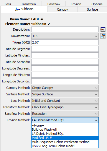
Figure 1. Selecting the surface erosion method for a subbasin element.

The parameters for each erosion method are presented on a separate Component Editor from the subbasin element editor. The "Erosion" editor is always shown next to the "Baseflow" editor. The information shown on the erosion editor will depend on which method is currently selected.

Build-up Wash-off

The build-up wash-off erosion method is designed for urban environments. In these environments, sediment accumulates in street curbs due to wind deposit and erosion from pervious areas adjacent to the curbs. The sediment accumulates during dry periods between storms. During a storm, the accumulated sediment is flushed from the street curbs by stormwater runoff. The method may optionally include street sweeping operations designed to mechanically remove accumulated sediment. A typical example of source data for parameterizing the method is Breault et al. (2005) though data sources should always be recognized as highly local. The Component Editor is shown in Figure 2.

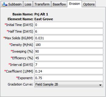
Figure 2. Build-up wash-off erosion method editor at a subbasin element.

The initial time is an initial condition for the method. It specifies the number of days since the last sweeping operation when the simulation begins.

The half time specifies the number of days required for half of the maximum solids to accumulate in the street curb under continuously dry conditions.

The maximum solids amount is the limit to the accumulated sediment in the street curb under continuously dry conditions. Sediment will not exceed this amount even if there is no precipitation for an extended period of time.

This erosion method includes four parameters to describe the street sweeping operations within the subbasin. The density specifies the total length of street curb whether or not the curb is subject to sweeping operations. The density should consider whether the street has curbs on one side or both sides of the street. The sweeping percentage specifies the percentage of the curb length subject to sweeping. The percentage should account for the possible presence of parked cars which result is missed curb. The efficiency percentage specifies the efficiency of the sweeping equipment at removing accumulated sediment. Finally, the interval specifies the number of days between scheduled sweeping operations.

The wash-off coefficient determines how quickly the accumulated sediment is removed from the street curb during a storm event.

The exponent is used to distribute the sediment load into a time-series sedigraph. A small value flattens the sedigraph compared to the hydrograph. A large value heightens the sedigraph compared to the hydrograph.

The gradation curve defines the distribution of the total sediment load into grain size classes and subclasses. The gradation curve is defined as a diameter-percentage function in the Paired Data Manager. The current functions are shown in the selection list. If there are many different functions available, you may wish to choose a function from the selector accessed with the paired data button next to the selection list. The selector displays the description for each function, making it easier to select the correct one.

Modified USLE

The modified USLE method (Williams, 1975) was adapted from the original Universal Soil Loss Equation. The original equation was based on precipitation intensity, and consequently could not differentiate between storms with low or high infiltration. With high infiltration, there is little surface runoff and little accompanying surface erosion. Conversely, low infiltration events have relatively more surface runoff and consequently more surface erosion. The modifications to the original USLE equation changed the formulation to calculate erosion from surface runoff instead of precipitation. The other components of the original formulation remained the same. The method works best in agricultural environments where it was developed. However, some users have adapted it to construction and urban environments. The Component Editor is shown in Figure 3.

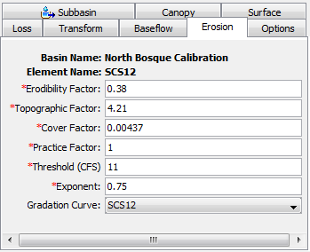
Figure 3. Modified USLE erosion method editor at a subbasin element.

The erodibility factor describes the difficulty of eroding the soil. The factor is a function of the soil texture, structure, organic matter content, and permeability. Typical values range from 0.05 for unconsolidated loamy sand to 0.75 for silty and clayey loam soils.

The topographic factor describes the susceptibility to erosion due to length and slope. It is based on the observation that long slopes have more erosion than short slopes, and steep slopes have more erosion than flat slopes. Typical values range from 0.1 for short and flat slopes to 10 for long or steep slopes.

The cover factor describes the influence of plant cover on surface erosion. Bare ground is the most susceptible to erosion while a thick vegetation cover significantly reduces erosion. Typical values range from 1.0 for bare ground, to 0.1 for fully mulched or covered soils, to as small as 0.0001 for forest soils with a well developed soil O horizon under a dense tree canopy.

The practice factor describes the effect of specific soil conservation practices, sometimes called best management practices. Agricultural practices could include strip cropping, terracing, or contouring. Construction and urban practices could include silt fences, hydro seeding, and settling basins. It is difficult to establish general ranges for these practices as they are usually highly specific.

Only some precipitation events will cause surface erosion. The threshold can be used to set the lower limit for runoff events that cause erosion. Events with a peak flow less than the threshold will have no erosion or sediment yield.

The exponent is used to distribute the sediment load into a time-series sedigraph. A small value flattens the sedigraph compared to the hydrograph. A large value heightens the sedigraph compared to the hydrograph.

The gradation curve defines the distribution of the total sediment load into grain size classes and subclasses. The gradation curve is defined as a diameter-percentage function in the Paired Data Manager. The current functions are shown in the selection list. If there are many different functions available, you may wish to choose a function from the selector accessed with the paired data button next to the selection list. The selector displays the description for each function, making it easier to select the correct one.

LA Debris Method EQ1 

The Los Angeles District Debris Method - Equation 1 (Gatwood et al., 2000) was developed from statistical analysis of data from watersheds with an area from 0.1 mi² to 3.0 mi². The equation was developed based on 349 observations from 80 watersheds located in Southern California. All factors in the equation were significant at the 0.99 level of confidence. The LA Debris Method EQ 1 works best in arid or semi arid regions of Southern California where it was developed. The Component Editor is shown in Figures 4 and 5.

Figure 4. LA Debris Method EQ 1 editor with User-Specified Fire Factor Method.

Figure 5. LA Debris Method EQ 1 editor with Pak & Lee Fire Factor Method.

The adjustment-transposition (A-T) factor describes the difference in geomorphology between the subject watershed and the original watershed from which the regression equation was generated. This factor considers the surficial geology, soils, hillslope, and channel morphology. Watersheds of the San Gabriel Mountains from which the regression equation was developed have an A-T factor of 1.0. Watersheds in areas with higher debris potential would have an A-T factor greater than 1.0, while areas of lesser debris yield capacity would have an A-T factor less than 1.0.

The relief ratio describes the susceptibility to debris yield due to length and slope. It is based on the difference in elevation between the highest point in the watershed (measured at the end of the longest stream) and the lowest point (at the debris collection site) and dividing the difference between these two location by the maximum stream length as measured along the longest stream.

The fire factor method has two options including the User-Specified Fire Factor for event simulation and the Pak & Lee Fire Factor for continuous simulation.  The fire factor describes the occurrence of wildfire on surface erosion. Information about the User-Specified Fire Factor is presented in Figure 2 (page 17) of the Los Angeles District Debris Method (Gatwood et al., 2000). Typical values range from 6.5 for within 1-year since 100% burn to 3.0 for more than 10-years since 100% burn. In order to apply the Pak & Lee Fire Factor method, two additional input parameters are required. The first one is the date which is the finish date of the most recent wildfire and the second one is the burn percentage of subbasin.  

The flow rate threshold can be used to divide storm events for the continuous simulation by setting the lower limit for direct runoff flow rate. A debris flow event starts when the direct runoff is above the flow rate threshold. The event ends when direct runoff falls below the threshold.

The exponent is used to distribute the sediment load into a time-series sedigraph. A small value flattens the sedigraph compared to the hydrograph. A large value heightens the sedigraph compared to the hydrograph.

The gradation curve defines the distribution of the total sediment load into grain size classes and subclasses. The gradation curve is defined as a diameter-percentage function in the Paired Data Manager. The current functions are shown in the selection list. If there are many different functions available, you may wish to choose a function from the selector accessed with the paired data button next to the selection list. The selector displays the description for each function, making it easier to select the correct one.

LA Debris Method EQ 2-5

The Los Angeles District Debris Method - Equation 2 through 5 (Gatwood et al., 2000) was developed from statistical analysis of data from watersheds with an area from 3.0 to 200.0 mi². This method may also be used for drainage areas less than 3 mi².  The Los Angeles District Debris Method EQ 2-5 works best in arid or semi arid regions of Southern California where it was developed. The Component Editor is shown in Figures 6 and 7.

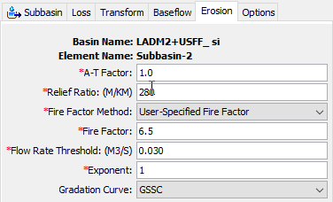
Figure 6. LA Debris Method EQ 2-5 editor with User-Specified Fire Factor Method.

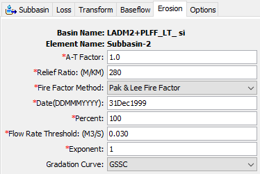
Figure 7. LA Debris Method EQ 2-5 editor with Pak & Lee Fire Factor Method.

The adjustment-transposition (A-T) factor describes the difference in geomorphology between the subject watershed and the original watershed from which the regression equation was generated. This factor considers the surficial geology, soils, hillslope, and channel morphology. Watersheds of the San Gabriel Mountains from which the regression equation was developed have an A-T factor of 1.0. Watersheds in areas with higher debris potential would have an A-T factor greater than 1.0, while areas of lesser debris yield capacity would have an A-T factor less than 1.0.

The relief ratio describes the susceptibility to debris yield due to length and slope. It is based on the difference in elevation between the highest point in the watershed (measured at the end of the longest stream) and the lowest point (at the debris collection site) and dividing the difference between these two location by the maximum stream length as measured along the longest stream.

The fire factor method has two options including the User-Specified Fire Factor for event simulation and the Pak & Lee Fire Factor for continuous simulation.  The fire factor describes the occurrence of wildfire on surface erosion. Information about the User-Specified Fire Factor is presented in Figure 2 (page 17) of the Los Angeles District Debris Method (Gatwood et al., 2000). Typical values range from 6.5 for within 1-year since 100% burn to 3.0 for more than 10-years since 100% burn. In order to apply the Pak & Lee Fire Factor method, two additional input parameters are required. The first one is the date which is the finish date of the most recent wildfire and the second one is the burn percentage of subbasin.  

The flow rate threshold can be used to divide storm events for the continuous simulation by setting the lower limit for direct runoff flow rate. A debris flow event starts when the direct runoff is above the flow rate threshold. The event ends when direct runoff falls below the threshold.

The exponent is used to distribute the sediment load into a time-series sedigraph. A small value flattens the sedigraph compared to the hydrograph. A large value heightens the sedigraph compared to the hydrograph.

The gradation curve defines the distribution of the total sediment load into grain size classes and subclasses. The gradation curve is defined as a diameter-percentage function in the Paired Data Manager. The current functions are shown in the selection list. If there are many different functions available, you may wish to choose a function from the selector accessed with the paired data button next to the selection list. The selector displays the description for each function, making it easier to select the correct one.

Multi-Sequence Debris Prediction Method (MSDPM) 

The Multi-Sequence Debris Prediction Method (Pak and Lee, 2008) was developed based on debris clean out data (1938 to 2002) obtained for 80 debris basins located in Southern California. The method can be used for the continuous debris yield simulation for relatively small watersheds from 0.1 mi² to 3.0 mi² in area. MSDPM is based on three main physical processes: the critical condition to entrained sediment, the transport capacity to move sediment toward the concentration point (debris basin), and the antecedent precipitation condition coupled with subsequent rainfall events. MSDPM works best in arid or semi arid regions of Southern California where it was developed. The Component Editor is shown in Figures 8 and 9.

Figure 8. Multi-Sequence Debris Prediction Method editor with User-Specified Fire Factor Method at a subbasin element.

Figure 9.  Multi-Sequence Debris Prediction Method editor with Pak & Lee Fire Factor Method at a subbasin element.

The adjustment-transposition (A-T) factor describes the difference in geomorphology between the subject watershed and the original watersheds from which the regression equations were generated. This factor considers the surficial geology, soils, and hillslope and channel morphology. Watersheds of the San Gabriel Mountains from which the regression equation was developed have an A-T factor of 1.0. Watersheds in areas with higher debris potential would have an A-T factor greater than 1.0, while areas of lesser debris yield capacity would have an A-T factor less than 1.0.

The relief ratio describes the susceptibility to debris yield due to length and slope. It is based on the difference in elevation between the highest point in the watershed (measured at the end of the longest stream) and the lowest point (at the debris collection site) and dividing the difference between these two locations by the maximum stream length as measured along the longest stream.

The threshold maximum 1-hr rainfall intensity (TMRI) describes the critical condition for entrainment of sediment. Not all rainfall events can generate sediment because some minimum energy is needed to entrain sediment particles. Therefore, rainfall events are screened by TMRI as a calibration factor to select those events where effective rainfall exceeds the critical value to entrain sediment particles.

The total minimum rainfall amount (TMRA) describes the transport capacity to move sediment to the concentration point. Not all rainfall events can lead to significant sediment transport. Once sediment has become entrained, a certain amount of additional energy is needed to move the sediment to the concentration point. Therefore, rainfall events are screened again by TMRA as a calibration factor to select effective rainfall events that can provide the required energy.

The fire factor method has two options including the User-Specified Fire Factor for event simulation and the Pak & Lee Fire Factor for continuous simulation.  The fire factor describes the occurrence of wildfire on surface erosion. The information for the User-Specified Fire Factor is presented in Figure 2 (page 17) of the Los Angeles District Debris Method (Gatwood et al., 2000). Typical values range from 6.5 for within 1-year since 100% burn to 3.0 for more than 10-years since 100% burn. In order to apply Pak & Lee Fire Factor method, two additional pieces of information are required. The first one is the finish date of the most recent wildfire and the second one is the burn percentage of subbasin.  

The flow rate threshold can be used to divide storm events for the continuous simulation by setting the lower limit for direct runoff flow rate. A debris flow event starts when the direct runoff is above the flow rate threshold. The event ends when direct runoff falls below the threshold.

The exponent is used to distribute the sediment load into a time-series sedigraph. A small value flattens the sedigraph compared to the hydrograph. A large value heightens the sedigraph compared to the hydrograph.

The gradation curve defines the distribution of the total sediment load into grain size classes and subclasses. The gradation curve is defined as a diameter-percentage function in the Paired Data Manager. The current functions are shown in the selection list. If there are many different functions available, you may wish to choose a function from the selector accessed with the paired data button next to the selection list. The selector displays the description for each function, making it easier to select the correct one.

USGS Long-Term Debris Model 

The USGS Long-Term Debris Model (Gartner et al., 2014) was developed from a database of 344 volumes of sediment deposited by debris flows and sediment-laden floods with no time limit since the most recent fire.  The sediment volume dataset represents a broad sample of conditions found in Ventura, Los Angeles and San Bernardino Counties, California. The Component Editor for this method is shown in Figure 10.

Figure 10. USGS Long-Term Debris Model editor at a subbasin element.

The relief describes the amount of energy available for transporting material down slope. It is the maximum amount of relief (maximum elevation minus minimum elevation) found within the watershed. 

The date is the finish date of the most recent wildfire.   

The burn area is the total area of watershed burned by the most recent wildfire.

The flow rate threshold can be used to divide storm events for the continuous simulation by setting the lower limit for direct runoff flow rate. A debris flow event starts when the direct runoff is above the flow rate threshold. The event ends when direct runoff falls below the threshold.

The exponent is used to distribute the sediment load into a time-series sedigraph. A small value flattens the sedigraph compared to the hydrograph. A large value heightens the sedigraph compared to the hydrograph.

The gradation curve defines the distribution of the total sediment load into grain size classes and subclasses. The gradation curve is defined as a diameter-percentage function in the Paired Data Manager. The current functions are shown in the selection list. If there are many different functions available, you may wish to choose a function from the selector accessed with the paired data button next to the selection list. The selector displays the description for each function, making it easier to select the correct one.

USGS Emergency Assessment Debris Model 

The USGS Emergency Assessment Debris Model (Gartner et al., 2014) was developed from a subset of the complete dataset consisting of 92 volumes of sediment deposited by debris flows within two years of a fire.  The sediment volume dataset represents a broad sample of conditions found in Ventura, Los Angeles and San Bernardino Counties, California. The Component Editor for this method is shown in Figure 11.

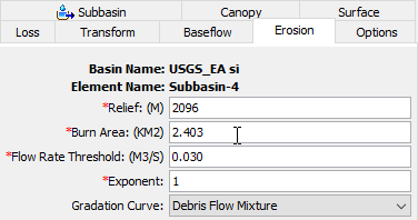
Figure 11. USGS Emergency Assessment Debris Model editor at a subbasin element.

The relief describes the amount of energy available for transporting material down slope. It is the maximum amount of relief (maximum elevation minus minimum elevation) found within the watershed. 

The burn area is the watershed area burned at moderate and high severity.

The flow rate threshold can be used to divide storm events for the continuous simulation by setting the lower limit for direct runoff flow rate. A debris flow event starts when the direct runoff is above the flow rate threshold. The event ends when direct runoff falls below the threshold.

The exponent is used to distribute the sediment load into a time-series sedigraph. A small value flattens the sedigraph compared to the hydrograph. A large value heightens the sedigraph compared to the hydrograph.

The gradation curve defines the distribution of the total sediment load into grain size classes and subclasses. The gradation curve is defined as a diameter-percentage function in the Paired Data Manager. The current functions are shown in the selection list. If there are many different functions available, you may wish to choose a function from the selector accessed with the paired data button next to the selection list. The selector displays the description for each function, making it easier to select the correct one.