Parameter estimation is the process of adapting a general model to a specific watershed. Some parameters can be estimated directly from field measurements. For example, the area that must be entered for a subbasin element can be measured directly in the field using standard surveying procedures or from maps developed through surveying. Other parameters can be estimated indirectly from field measurements. In this case, the field measurement does not result in a value that can be input directly to the program. However, the field measurement can provide a strong recommendation for a parameter in the program based on previous experience. For example, measurements of soil texture are correlated with parameters such as hydraulic conductivity. Finally, there are parameters that can only be estimated by comparing computed results to observations such as measured streamflow. Even for parameters of the first two types, there is often enough uncertainty in the true parameter value to require some adjustment of the estimates in order for the model to closely follow the observed streamflow.

The quantitative measure of the goodness-of-fit between the computed result from the model and the observed flow is called the objective function. Different objective functions measure the degree of variation between computed and observed hydrographs in different ways. Some functions report a value that decreases as the agreement between simulated and observed increases, and some do the opposite, increasing as goodness-of-fit increases. The key to automated parameter estimation is a search method for adjusting parameters to direct the objective function value towards better goodness-of-fit, and find optimal parameter values. An optimal value for the objective function is obtained when the parameter values best able to reproduce the observed hydrograph are found. Constraints are set to ensure that unreasonable parameter values are not used.

Optimization trials are one of the components that can compute results. Each trial is composed of a basin model, meteorologic model, and time control information. The trial also includes selections for the objective function, search method, and parameters to be adjusted in order to find an optimal model. A variety of result graphs and tables are available from the Watershed Explorer for evaluating the quality of the results.

The iterative parameter estimation procedure used by the program is often called optimization. Initial values for all parameters are required at the start of the optimization trial time window. A hydrograph is computed at a target element by computing all of the upstream elements. The target must have an observed hydrograph for the time period over which the objective function will be evaluated. Only parameters for upstream elements can be estimated. The value of the objective function is computed at the target element using the computed and observed hydrographs. Parameter values are adjusted by the search method and the hydrograph and objective function for the target element are recomputed. This process is repeated until the value of the objective function is sufficiently small, or the maximum number of iterations is reached. Results can be viewed after the optimization trial is complete.

Creating a New Optimization Trial

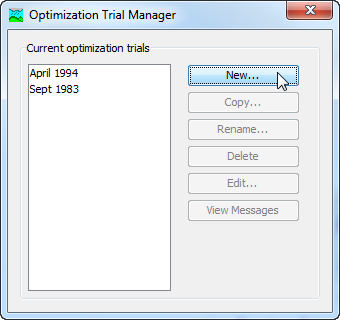
A new optimization trial is created using a wizard that helps you navigate the steps to creating a new trial. There are two ways to access the wizard. The first way to access the wizard is to click on the Compute menu and select the Create Compute | Optimization Trial command; it is only enabled if at least one basin model and meteorologic model exist. The wizard will open and begin the process of creating a new optimization trial. The second way to access the wizard is from the Optimization Trial Manager. Click on the Compute menu and select the Optimization Trial Manager command. The Optimization Trial Manager will open and show any trials that already exist. Press the New… button to access the wizard and begin the process of creating an optimization trial, as shown in Figure 1.

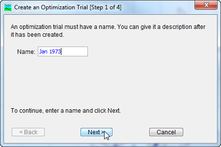
The first step of creating an optimization trial is to provide the name for the new trial (Figure 2). A default name is provided for the new optimization trial; you can use the default or replace it with your own choice. After you finish creating the trial you can add a description to it. If you change your mind and do not want to create a new optimization trial, you can press the Cancel button at the bottom of the wizard or the X button in the upper right corner of the wizard. The Cancel button can be pressed at any time you are using the wizard. Press the Next> button when you are satisfied with the name you have entered and are ready to proceed to the next step.

The second step of creating an optimization trial is to select a basin model. All of the basin models that are currently part of the project are displayed in alphabetical order. By default the first basin model in the table is selected. The selected basin model is highlighted. You can use your mouse to select a different basin model by clicking on it in the table of available choices. You can also use the arrow keys on your keyboard to select a different basin model. Press the Next> button when you are satisfied with the basin model you have selected and are ready to proceed to the next step. Press the <Back button if you wish to return to the previous step and change the name for the new optimization trial.

The third step of creating an optimization trial is to select an element where there is observed flow. The element is where the objective function will be evaluated. You will only be able to perform parameter estimation at, or upstream of the selected element. The elements in the selection list come from the basin model used in the simulation run that was selected in the previous step. By default the first element in the table is selected. The selected element is always highlighted. You can use your mouse to select a different element by clicking on it in the table of available choices. You can also use the arrow keys on your keyboard to select a different element. Press the Next> button when you are satisfied with the element you have selected and are ready to proceed to the next step. Press the <Back button if you wish to return to the previous step and change the selected basin model for the new optimization trial.

The fourth step of creating an optimization trial is to select a meteorologic model. All of the meteorologic models that are currently part of the project are displayed in alphabetical order. By default the first meteorologic model in the table is selected. The selected meteorologic model is highlighted. You can use your mouse to select a different meteorologic model by clicking on it in the table of available choices. You can also use the arrow keys on your keyboard to select a different meteorologic model. You are responsible for selecting a basin model in step two and a meteorologic model in this step that will successfully combine to compute results. Press the Finish button when you are satisfied with the name you have entered, the basin model and element you selected, the meteorologic model you selected, and are ready to create the optimization trial. Press the <Back button if you wish to return to the previous step and select a different element for comparing computed results and computing the objective function.

Copying an Optimization Trial

There are two ways to copy an optimization trial. Both methods for copying a trial create an exact duplicate with a different name. Once the copy has been made it is independent of the original and they do not interact.

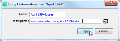
The first way to create a copy is to use the Optimization Trial Manager, which is accessed from the Compute menu. Select the optimization trial you wish to copy by clicking on it in the list of current optimization trials. The selected trial is highlighted after you select it. After you select a trial you can press the Copy… button on the right side of the window. The Copy Optimization Trial window (Figure 3) will open where you can name and describe the copy that will be created. A default name is provided for the copy; you can use the default or replace it with your own choice. A description can also be entered; if it is long you can use the button to the right of the description field to open an editor. When you are satisfied with the name and description, press the Copy button to finish the process of copying the selected optimization trial. You cannot press the Copy button if no name is specified. If you change your mind and do not want to copy the selected optimization trial, press the Cancel button or the X button in the upper right to return to the Optimization Trial Manager window.

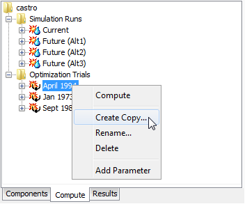
The second way to copy is from the "Compute" tab of the Watershed Explorer. Move the mouse over the optimization trial you wish to copy and press the right mouse button (Figure 4). A context menu is displayed that contains several choices including copy. Click the Create Copy… command. The Copy Optimization Trial window will open where you can name and describe the copy that will be created. A default name is provided for the copy; you can use the default or replace it with your own choice. A description can also be entered; if it is long you can use the button to the right of the description field to open an editor. When you are satisfied with the name and description, press the Copy button to finish the process of copying the selected optimization trial. You cannot press the Copy button if no name is specified. If you change your mind and do not want to copy the selected optimization trial, press the Cancel button or the X button in the upper right of the Copy Optimization Trial window to return to the Watershed Explorer.

Renaming an Optimization Trial

There are two ways to rename an optimization trial. Both methods for renaming a trial change its name and perform other necessary operations.

The first way to perform a rename is to use the Optimization Trial Manager, which you can access from the Compute menu. Select the optimization trial you wish to rename by clicking on it in the list of current optimization trials. The selected trial is highlighted after you select it. After you select a trial you can press the Rename… button on the right side of the window. The Rename Optimization Trial window (Figure 5) will open where you can provide the new name. If you wish you can also change the description at the same time. If the new description will be long, you can use the button to the right of the description field to open an editor. When you are satisfied with the name and description, press the Rename button to finish the process of renaming the selected optimization trial. You cannot press the Rename button if no name is specified. If you change your mind and do not want to rename the selected simulation trial, press the Cancel button or the X button in the upper right of the Rename Optimization Trial window to return to the Optimization Trial Manager window.

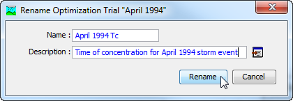
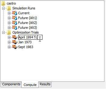
The second way to rename is from the "Compute" tab of the Watershed Explorer. Select the optimization trial you wish to rename by clicking on it in the Watershed Explorer; it will become highlighted. Keep the mouse over the selected trial and click the left mouse button again. The highlighted name will change to editing mode (Figure 6). You can then move the cursor with the arrow keys on the keyboard or by clicking with the mouse. You can also use the mouse to select some or all of the name. Change the name by typing with the keyboard. When you have finished changing the name, press the Enter key to finalize your choice. You can also finalize your choice by clicking elsewhere on the "Compute" tab. If you change your mind while in editing mode and do not want to rename the selected optimization trial, press the Escape key.

Deleting an Optimization Trial

There are two ways to delete an optimization trial. Both methods for deleting a trial remove it from the project and automatically delete previously computed results. Once a trial has been deleted it cannot be retrieved or undeleted.

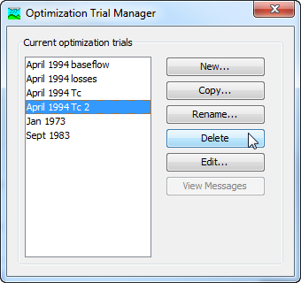
The first way to perform a deletion is to use the Optimization Trial Manager, which you can access from the Compute menu. Select the optimization trial you wish to delete by clicking on it in the list of current optimization trials. The selected trial is highlighted after you select it. After you select a trial you can press the Delete button on the right side of the window. A window will open where you must confirm that you wish to delete the selected trial as shown in Figure 7. Press the OK button to delete the trial. If you change your mind and do not want to delete the selected optimization trial, press the Cancel button or the X button in the upper right to return to the Optimization Trial Manager window.

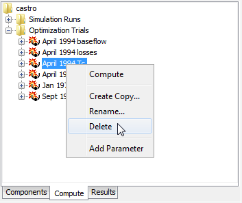
The second way to delete is from the "Compute" tab of the Watershed Explorer. Select the optimization trial you wish to delete by clicking on it in the Watershed Explorer; it will become highlighted (Figure 8). Keep the mouse over the selected trial and click the right mouse button. A context menu is displayed that contains several choices including delete. Click the Delete command. A window will open where you must confirm that you wish to delete the selected trial. Press the OK button to delete the trial. If you change your mind and do not want to delete the selected optimization trial, press the Cancel button or the X button in the upper right to return to the Watershed Explorer.

Selecting Components

One of the principal tasks when creating an optimization trial using the wizard is the selection of the components that will be used to compute optimization results. The components include the basin model and the hydrologic element in the basin model where the objective function will be computed. The components also include the meteorologic model. These components are selected when creating a new optimization trial with the wizard. However, you can change the basin model and meteorologic model you wish to use at any time using the Component Editor for the optimization trial. Access the Component Editor from the "Compute" tab of the Watershed Explorer (Figure 9). If necessary, click on the "Optimization Trials" folder to expand it and view the available optimization trials. The Component Editor contains a basin model selection list that includes all of the basin models in the project where the basin model has at least one element with observed flow. The Component Editor also contains a meteorologic model selection list that includes all of the meteorologic models in the project. The Search and Objective tabs of the Optimziation Trial Component Editor are discuss in the following sections.

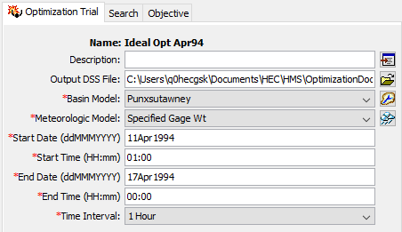
Entering a Time Window

You must enter a start date and time and an end date and time for the optimization trial. The time control information is not specified in the wizard used to create the optimization trial. The time control information must be entered after the trial is created using the Component Editor for the optimization trial (Figure 9). Enter the start date using the indicated format for numeric day, abbreviated month, and four-digit year. Enter the end date using the same format. The start time and end time are entered using 24-hour time format. Choose a time interval from the available options which range from 1 minute up to 1 day. Finally, the start time and end time must each be an integer number of time intervals after the beginning of the day.

Search Methods: Deterministic

Two deterministic search methods are available for optimizing the objective function and returning optimal parameter values. The univariate method evaluates and adjusts one parameter during the optimization simulation, the user can choose only one parameter for the program to adjust when the univariate method is selected. The Simplex method uses a downhill simplex to evaluate all parameters simultaneously and determine which parameter to adjust. The default method is the simplex method, at least two parameters must be selected when the simplex method is chosen.

Selecting the search method for the optimization trial is accessed from the "Compute" tab of the Watershed Explorer in the optimization trial Component Editor. Click on the optimization trial node to display the Component Editor for the optimization trial (Figure 9). If necessary, click on the "Optimization Trials" folder to expand it and view the available optimization trials in the project.

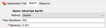
Two methods are provided for controlling the search process, the Univariate or Simplex methods. Both search methods function by iteratively adjusting parameter values to decrease the objective function value (increase if the goal is maximization); each parameter adjustment is termed an "iteration." The tolerance determines the change in the objective function value between two successive iterations that will terminate the search; when the objective function changes less than the specified tolerance, the search terminates. The maximum number of iterations also can be used to limit the search. The search will stop when the maximum number of iterations is reached regardless of changes in the objective function value or the quality of the estimated parameters. The tolerance and maximum iterations are both entered on the Search tab within the optimization trial Component Editor (Figure 10). Defaults are provided for both criteria. The initial default values depend on the selected search method.

Search Methods: Stochastic

Markov Chain Monte Carlo (MCMC) is the stochastic search method available in HEC-HMS. The general principle of MCMC optimization is this: the algorithm seeks to visit the plausible parameter sets in a parameter space by a random walk, and visit parameter sets that are more likely to have created the observed dataset more often. MCMC search proceeds by generating a sequence of parameter values by making random transitions from one state of a Markov Chain to another using a proposal distribution. Each state is a set of model parameter values for the parameters being optimized. If the present state (parameter values) of the Markov Chain implies good agreement between the simulated and observed data, then the iteration is less likely to make large jumps away from the present state. This produces repeated samples from a region of the parameter space that is associated with higher likelihood that the parameter set produced the observed values. If the agreement is not good, then larger random leaps across the parameter space are likely to occur. Multiple chains, which are initialized with different starting conditions, are used to assess whether the samples have escaped the starting conditions and have begun to draw samples from the highest-likelihood regions of the parameter space, which are unknown at the outset. The state of drawing from the highest-likelihood region of the parameter space is called equilibrium. It is desirable to have many samples from this region in order to characterize the statistical properties of the parameters associated with this high-likelihood space.

The MCMC search requires additional parameterization in order to operate (Figure 11). "Pool Size" controls the number of independent Markov Chains used in the simulation. "Initial Sample" controls the number of burn-in samples to be taken before beginning to assess sample convergence. "Min Iterations" and "Max Iterations" controls the allowable range of iterations for the simulation. "Convergence" allows the user to set the value for the Gelman-Rubin statistic that discriminates between pre- and post-equilibrium samples (the default value of 1.2 is generally sufficient; higher discrimination would be enforced using a lower number not lower than 1.0). "Equilibrium Sample" controls the number of samples drawn after the simulation has achieved a state of equilibrium.

Selecting the search method for the optimization trial is accessed from the "Compute" tab of the Watershed Explorer in the optimization trial Component Editor. Click on the optimization trial node to display the Component Editor for the optimization trial (Figure 9). If necessary, click on the "Optimization Trials" folder to expand it and view the available optimization trials in the project.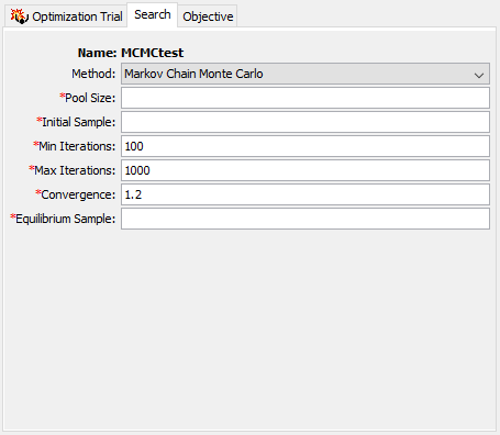



Figure 11. The Search tab of the Component Editor for Markov Chain Monte Carlo requires additional parameterization of the search settings from those required of deterministic optimizations.

Objective Function: Deterministic Optimization

The objective function measures the goodness-of-fit between the computed outflow and observed streamflow at the selected element. For the minimization goal, there are fourteen different goodness-of-fit functions which decrease as agreement between simulated and observed increases. The maximization goal can be used in two different ways: to maximize an element property such as flow volume or peak discharge, reservoir stage, etc., or to maximize a goodness-of-fit statistic which increases in value as goodness-of-fit increases. See Table 1 for minimization goal objective functions, and Table 2 for maximization goal objective functions.

Table 1. Minimization Goal Objective Functions and their motivation.

Table 2.Maximization Goal Objective Functions and their motivation.

Maximization of an element time-series statistic, such as flow volume, peak discharge or especially peak reservoir pool elevation, is used in conjunction with hazard analyses such as those required for dam safety studies. A particularly important optimization is when the trial is used in conjunction with the HMR 52 Storm precipitation method to maximize a statistic. The optimization trial automatically adjusts HMR 52 Storm parameters during the maximization trial, which replaces the need for many manual iterations of running simulations to determine the optimal HMR52 Storm parameter set.

Figure 12 shows the "Objective" tab for the optimization trial Component Editor. Maximization is set for the "Goal" of the optimization. The "Location" is the basin model element where the user wants the optimization trial to maximize the selected statistic. Any element within the basin model can be selected. The Time-Series drop down list provides options based on the type of element selected for the location. If a reach, subbasin, or junction is selected, then discharge is the only available time-series. If a reservoir element is selected, then the user can choose between discharge and pool elevation. The "Statistic" is the computed result that is maximized during the optimization trial. When discharge is selected as the time-series, then the user can choose a statistic of Discharge Volume or Peak Discharge. When pool elevation is selected as the time-series, then the only statistic option is Peak Elevation.

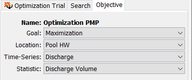
Figure 12. Objective tab for an optimization trial with the Goal set to Maximization.

The HMR 52 Storm parameters that can be adjusted in the optimization trial are Orientation, Area, X and Y Coordinates, and the Peak Intensity Period. Figure 13 shows the the Parameter tab within the optimization trial Component Editor. The Precipitation Parameters option is chosen for the Element (the precipitation parameters are global to all subbasins in the basin model). The parameter list includes all parameter available to be adjusted during the optimization trial. The initial value is the value specified in the meteorologic model referenced by the optimization trial, the user can change the initial value. Default minimum and maximum values are set by the program, the user should override these values with information about the watershed. By default, the minimum and maximum x and y coordinates are defined using coordinates from the subbasin GIS features.

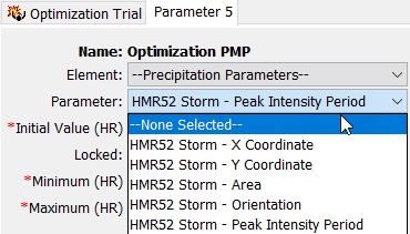
Figure 13. Parameter options for an optimization trial configured to work with a HMR 52 Storm meteorologic model.

Select the objective function method for the optimization trial on the Component Editor for the objective function (Figure 14). Access the Component Editor from the "Compute" tab of the Watershed Explorer. If necessary, click on the "Optimization Trials" folder to expand it and view the available optimization trials in the project. Click on the optimization trial node to expand it and see the objective function node. Click on the objective function node to view the editor. Select the "Objective" tab within the Component Editor.

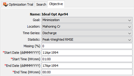
Figure 14. The Objective tab of the Component Editor for deterministic optimizations allows for specification of the goal for optimization, including the time window over which the objective function will be evaluated. The user is also able to specify whether a minimization or a maximization of the objective function is desired. The valid choices for objective function are affected by the selection of a goal type.

An element with observed flow was selected at the time the optimization trial was created. This is the location where the objective function will be evaluated. You can change the element location at any time using the Component Editor for the objective function. The selection list shows all of the elements with observed flow in the basin model selected for the optimization trial. Select a different element in the list to change where the objective function will be evaluated. Recognize that parameters can only be estimated at locations upstream of the selected element. Changing the location will change which parameters can be estimated.

In general, the observed flow record at the selected element location should not contain any missing data. However, you can specify the amount of missing data in the observed flow that will be permitted. Specify the amount that may be missing as a percentage. The program will check the observed flow record and only perform the optimization if the percentage of missing flow in the record is less than the specified amount. Time steps with missing data are ignored when computing the value of the objective function. The default amount of missing flow is 0.0 percent.

The objective function is evaluated over a specified time window. The time window cannot begin before the start time of the optimization trial. Also, the time window cannot end after the end time of the optimization trial. However, you have the option of changing the time window to be narrower than the one specified for the whole optimization trial. By default, the start and end time for the objective function will default to the time window of the optimization trial.

Objective Function: Stochastic Optimization

Only one goal and objective function are available for MCMC optimization: minimization goal with the Sum of Squared Residuals objective function. This combination allows the MCMC algorithm to assess the likelihood that a particular parameter set is the one that produced the observed data. Figure 15 shows this selection, which is populated by default when MCMC is selected.

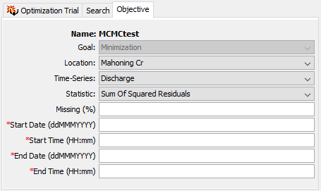
Figure 15. The Objective tab of the Component Editor for MCMC optimization only allows for a minimization goal, and a single statistic, Sum of Squared Residuals.

Adding and Deleting Parameters

The parameters that will be automatically estimated must be at the selected element location or upstream of it in the element network. When the selected location is changed, elements will be automatically deleted if they are not upstream of the newly selected location. Parameters that can be chosen for estimation are a selected set of the canopy, surface, lossrate, transform, baseflow parameters in the subbasin, and routing parameters in the reach. Parameters that should be strictly measured in the field are not allowed to be estimated. For example, it is not permissible to estimate subbasin area or a reach length.

Care must be taken when selecting parameters for estimation. While it is possible to select the same parameter more than once, it is not recommended. In this scenario, the search method attempts to improve estimates by adjusting the same parameter value at different and sometimes conflicting points in the search. This can lead to a so-called blocking condition where the search method cannot accurately determine how to adjust parameters to improve the objective function and less than optimal results are achieved.

Care must also be taken when selecting parameters at elements upstream of the observed flow location. It is possible to select multiple parameters that have similar affects on the computed hydrograph at the evaluation location. In this case, adjustments to one parameter can off set adjustments in others. For example, estimates of the time of concentration at multiple subbasins upstream of the evaluation location often result in poor results. Special parameters called scale factors have been included that adjust all similar parameters upstream of the evaluation location together in the same direction. However, care is still required even with this special scaling. Scale factors can be used specifying the optimization location at a downstream location from the elements to be scaled (e.g. a junction), adding a parameter, and selecting - All Subbasins - as the element of interest. Then, the parameter entry will allow for selection of scale factors, as in Figure 16.

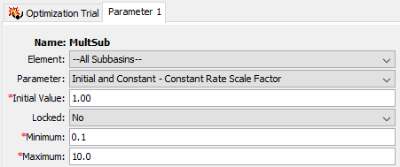
Figure 16. Parameter specification invoking scale factors.

Add a new parameter to an optimization trial using the Watershed Explorer. Move the mouse over the optimization trial and press the right mouse button (Figure 17). A context menu is displayed that contains several choices including adding a parameter. Click the Add Parameter command. The subbasin canopy parameters that can be added are shown in Table 3. Subbasin surface parameters are shown in Table 4 and loss rate parameters are shown in Table 5. Subbasin transform parameters are shown in Table 6 and baseflow parameters are shown in Table 7. Reach routing parameters that can be added are shown in Table 8.

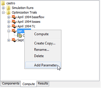
Figure 17. Adding a parameter to an optimization trial.

Delete a parameter from an optimization trial using the Watershed Explorer. Select the parameter you wish to delete by clicking on it in the Watershed Explorer; it will become highlighted. Keep the mouse over the selected parameter and click the right mouse button (Figure 18). A context menu is displayed that contains several choices including deleting a parameter. Click the Delete Parameter command.

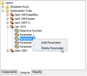
Figure 18. Deleting a selected parameter from an optimization trial.

Table 3. Subbasin canopy parameters available for optimization.

Table 4. Subbasin surface parameters available for optimization.

Table 5. Subbasin loss rate parameters available for optimization.

Table 6. Subbasin transform parameters available for optimization.

Table 7. Subbasin baseflow parameters available for optimization.

Table 8. Reach routing parameters available for optimization.

Specifying Parameter Information

A variety of information must be specified for each optimization parameter in order for the search method to function. Select the parameter you wish to edit by clicking on it in the Watershed Explorer. Click on the optimization trial node to expand it. The first node under the optimization trial will be the objective function. Following the objective function will be a separate node for each parameter. Click on the desired node in the Watershed Explorer to view the Component Editor for the optimization.

Each optimization parameter must select the element where the desired parameter resides. All eligible subbasin and reach elements upstream of the objective function evaluation location are shown in the selection list. Eligible subbasins are those using the methods listed in Table 3, Table 4, Table 5, Table 6, and Table 7. Eligible reaches are those using the methods listed in Table 8. Choosing an element from the list will update the list of available parameters based on the methods in use at that selected element. You may also have the choice of selecting the "All Subbasins" option in order to apply scale factors.

Each optimization parameter must select a specific parameter for the chosen element. The available choices are shown in the selection list. Once you make a choice from the list, the remainder of the data in the Component Editor will become available for use (Figure 19).

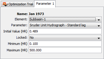
Figure 19. Specifying properties for a parameter in an optimization trial.

The initial value is the starting point for the parameter estimation process. The search method will begin searching from that point for optimal parameter values. The default initial value is the parameter value in the basin model that was selected for the optimization trial. You may change the initial value without affecting the basin model.

It is possible to lock a parameter. When a parameter is locked, the initial value is used and no adjustments are made during the search process.

The minimum parameter value can be used to narrow the lower end of the range of values that will be used by the search method. Likewise, the maximum parameter value can be used to narrow the upper end of the range of values that will be used by the search method. A good source of information for narrowing the search range is preliminary estimates from field measurements or manual calibration. Default values for the minimum and maximum are provided based on physical and numerical limits. The search may continue outside the specified range. When it does so, a penalty is applied that is proportional to the distance outside the specified range. The penalty nudges the search for optimal parameter values back to the range between the specified minimum and maximum.